Download
1 / 47
470 likes | 494 Vues
Learn about memoryless property, variance calculation by conditioning, conditional probability, and geometric distribution variance. Explore examples and recursive relationships in stochastic models.

E N D
Outline • memoryless property • geometric and exponential • V(X) = E[V(X|Y)] + V[E(X|Y)] • conditional probability 2
Memoryless Property of Geometric Distribution • X ~ Geo (p) • Y = the remaining life of given that X > 1 • Y = (X-1|X > 1) • P(Y = k) = P(X - 1 = k| X > 1) = = = = (1-p)k-1p = P(X = k) • Y ~ X • similarly, (X - m|X > m) ~ X for all m 1 • the memoryless property of Geometric 3
Memoryless Property of Exponent Distribution • X ~ exp(), P(X > s) = es, s > 0 • Y = the remaining life of given that X > t (> 0) • Y = (X-t|X > t) • P(Y > s) = P(X - t > s| X > t) = = = = es = P(X > s) • Y ~ X • the memoryless property of exponential 4
Finding Variance By Conditioning Proposition 3.1 of Ross • X & Y: two random variables • both V(X|Y) and E(X|Y) being random variables • well-defined E[V(X|Y)] & V[E(X|Y)] • E[V(X|Y)] = E[E(X2|Y)] - E[E2(X|Y)] • V[E(X|Y)] = E[E2(X|Y)] - E2[E(X|Y)] • E[V(X|Y)] + V[E(X|Y)] = E[E(X2|Y)] E2[E(X|Y)] = E[X2] E2[X] = V(X) 6
Variance of Random Sum • Xi's ~ i.i.d. random variables, mean & variance 2 • N: an integer non-negative random variable independent of Xi's, mean & variance 2 • S = 7
Variance of Random Sum • V(S) = E[V(S|N)] + V[E(S|N)] • V(S|N = n) = V( ) = n2 • E[V(S|N)] = E[N2] = 2E[N] = 2 • E(S|N = n) = E( ) = n • V[E(S|N)] = V[N] = 2V(N) = 22 • V(S) = 2+22 • not necessary to find the distribution of S 8
Variance of Geometric • X ~ Geo(p), 0 < p < 1 • IA = 1 if {X = 1} and IA = 0 if {X > 1} • P(IA = 1) = p and P(IA = 0) = 1-p = q • E[V(X|IA)] • V(X|X=1) = 0 • V(X|X>1) = V(1+X-1|X>1) = V(X-1|X>1) = V(X) • E[V(X|IA)] = p0 + qV(X) = qV(X) 9
Variance of Geometric Example 3.18 of Ross • V[E(X|IA)] • E[X|X=1] = 1 • E[X|X>1] = 1+ E[X-1| X>1] = • V[E(X|IA)] = E[E2(X|IA)] - E2[E(X| IA)] memoryless property of geometric 10
First Part of Example 3.26 of Ross • n men mixed their hats & randomly picked one • En: no matches for these n men • P(En) = ? • p1 = 0 • p2 = 0.5 12
First Part of Example 3.26 of Ross • n = 3 • M: correct hat for the first man • Mc: wrong hat for the first man • p3 = P(E3) = P(E3|M)P(M) + P(E3|Mc)P(Mc) = P(E3|Mc)P(Mc) • P(Mc) = 2/3 & P(E3|Mc) = 1/2 a A B b C c 13
First Part of Example 3.26 of Ross • n = 4 • M: correct hat for the first man • Mc: wrong hat for the first man • p4 = P(E4) = P(E4|M)P(M) + P(E4|Mc)P(Mc) = P(E4|Mc)P(Mc) • P(Mc) = 3/4 & P(E4|Mc) = ??? a A B b C c D d 14
First Part of Example 3.26 of Ross • P(E4|Mc) = ??? • Ca: C gets a • Cna: C does not get a • {E4|Mc} = {E4Ca|Mc} {E4Cna|Mc} • P(E4|Mc) = P(E4Ca|Mc) + P(E4Cna|Mc) a A B b C c D d 15
First Part of Example 3.26 of Ross • P(E4Cna|Mc) = P(E3) • P(E4Ca|Mc) = P(E4|CaMc)P(Ca|Mc) = P(E2)(2/3) a A B b C c D d 16
First Part of Example 3.26 of Ross • pn = P(En) = P(En|M)P(M) + P(En|Mc)P(Mc) = P(En|Mc)P(Mc) • Ha: the man whose hat picked by A picked A’s hat • Hna: the man whose hat picked by A did not pick A’s hat • P(En|Mc) = P(EnHna|Mc) + P(EnHa|Mc) • P(EnHna|Mc) = pn-1 • P(EnHa|Mc) = P(En|HaMc)P(Ha|Mc) = pn-2(1/n-1) • so • solving 17
Ex. #4 of WS#10 • #1. (Solve Exercise #4 of Worksheet #10 by conditioning, not direct computation.) Let X and Y be two independent random variables ~ geo(p). • (a). Find P(X = Y). • (b). Find P(X > Y). • (c). Find P(min(X, Y) > k) for k {1, 2, …}. • (d). From (c) or otherwise, Find E[min(X, Y)]. • (e). Show that max(X, Y) + min(X, Y) = X + Y. Hence find E[max(X, Y)]. 19
Ex. #4 of WS#10 • (a). different ways to solve the problem • by computation: • P(X = Y) = = = = = p/(2-p) 20
Ex. #4 of WS#10 • by conditioning: • P(X = Y|X = 1, Y = 1) = 1 • P(X = Y|X = 1, Y > 1) = 0 • P(X = Y|X > 1, Y = 1) = 0 • P(X = Y|X > 1, Y > 1) = P(X = Y) • P(X = Y) = P(X = 1, Y = 1)(1) + P(X > 1, Y > 1)P(X = Y) • P(X = Y) = p2 + (1p)2P(X = Y) i.e., P(X = Y) = p/(2p) 21
Ex. #4 of WS#10 • (b) P(X > Y) • by symmetry • P(X > Y) + P(X = Y) + P(X < Y) = 1 • P(X > Y) = P(X < Y) • P(X > Y) = = 22
Ex. #4 of WS#10 • by direct computation • P(X > Y) = 23
Ex. #4 of WS#10 • by conditioning • P(X > Y) = E[P(X > Y|Y)] • P(X > Y|Y = y) = P(X > y) = (1-p)y • E[P(X > Y|Y)] = E[(1-p)Y] 24
Ex. #4 of WS#10 • yet another way of conditioning • P(X > Y|X = 1, Y = 1) = 0 • P(X > Y|X = 1, Y > 1) = 0 • P(X > Y|X > 1, Y = 1) = 1 • P(X > Y|X > 1, Y > 1) = P(X > Y) • P(X > Y) = P(X > 1, Y = 1) + P(X > 1, Y > 1)P(X > Y) = (1-p)p + (1-p)2P(X > Y) • P(X > Y) = (1p)/(2p) 25
Ex. #5 of WS#10 • In the sea battle of Cape of No Return, two cruisers of country Landpower (unluckily) ran into two battleships of country Seapower. With artilleries of shorter range, the two cruisers had no choice other than receiving rounds of bombardment by the two battleships. Suppose that in each round of bombardment, a battleship only aimed at one cruiser, and it sank the cruiser with probability p in a round, 0 < p < 1, independent of everything else. The two battleships fired simultaneously in each round. 26
Ex. #5 of WS#10 • (a) Suppose that the two battleships first co-operated together to sink the same cruiser. Find the expected number of rounds of bombardment taken to sink both of the two cruisers. • pc= P(a cruiser was sunk in a round) = 1- P(a cruiser was not sunk in a round) = 1-(1-p)2 • expected number of rounds taken to sink a cruiser ~ Geo(pc) with mean = 1/pc • expected number of rounds taken to sink two cruisers = 2/pc 27
Ex. #5 of WS#10 • (b) Now suppose that initially the two battleships aimed at a different cruiser. They helped the other battleship only if its targeted cruiser was sunk before the other one. • (i) What is the probability that the two cruisers were sunk at the same time (with the same number of rounds of bombardment). 28
Ex. #5 of WS#10 • (b). (i). Ni = the number of rounds taken to sink the ith cruiser; Ni~ Geo (p); N1and N2 are independent. • ps= P(2 cruisers sunk at the same round) = P(N1 = N2) • discussed before 29
Ex. #5 of WS#10 • different ways to solve the problem • by computation: • P(N1 = N2) = = = = = p/(2-p) 30
Ex. #5 of WS#10 • by conditioning: • P(N1 = N2|N1 = 1, N2 = 1) = 1 • P(N1 = N2|N1 = 1, N2 > 1) = 0 • P(N1 = N2|N1 > 1, N2 = 1) = 0 • P(N1 = N2|N1 > 1, N2 > 1) = P(X = Y) • P(N1 = N2) = P(N1 = 1, N2 = 1)(1) + P(N1 = 1, N2 = 1)P(X = Y) • P(N1 = N2) = p2 + (1p)2P(N1 = N2) i.e., P(N1 = N2) = p/(2p) 31
Ex. #5 of WS#10 • (ii). Find the probability of taking k ({1, 2, …}) rounds to have the first sinking of a cruiser. • Y = the number of rounds to have the first sinking of a cruiser • different ways to find P(Y = k) 32
Ex. #5 of WS#10 • from the tail distribution • P(min(N1, N2) > k) = P(N1 > k, N2 > k) = P(N1 > k)P(N2 > k) = (1-p)2k • P(Y = k) = P(Y > k-1) - P(Y > k) = P(min(N1, N2) > k -1) - P(min(N1, N2) > k) = P(N1 > k –1, N2 > k –1) - P(N1 > k, N2 > k) = P(N1 > k –1)P(N2> k –1) - P(N1> k)P(N2> k) = (1p)2k-2 (1p)2k = (1p)2k-2p(2p) 33
Ex. #5 of WS#10 • from direct calculation • P(Y = k) = P(min(N1, N2) = k) = P(N1 = k, N2 = k) + P(N1 > k, N2 = k) + P(N1 = k, N2 > k) = P(N1 = k)P(N2 = k) + P(N1 > k)P(N2 = k) + P(N1 = k) P(N2 > k) = (1p)2k-2p2 + 2(1p)k(1p)k-1p = (1p)2k-2p(2p) 34
Ex. #5 of WS#10 • (iii). Find the expected number of rounds taken to have the first sinking of a cruiser • different ways to find E(Y) • by direct computation • E(Y) = = = = 35
Ex. #5 of WS#10 • from the tail distribution • E(Y) = = = = = = 36
Ex. #5 of WS#10 • by conditioning • E[min(N1, N2)|N1 = 1, N2 = 1] = 1 • E[min(N1, N2)|N1 = 1, N2 > 1] = 1 • E[min(N1, N2)|N1 > 1, N2 = 1] = 1 • E[min(N1, N2)|N1 > 1, N2 > 1] = 1 + E[min(N1, N2)] • E[min(N1, N2)] = 1 + (1-p)2 E[min(N1, N2)] • E[min(N1, N2)] = 37
Ex. #5 of WS#10 • (iv). Z = # of rounds taken to sink both cruisers; find E(Z) • by conditioning • E(Z|N1 = 1, N2 = 1) = 1 • E(Z|N1 = 1, N2 > 1) = 1 + E(N2’) • E(Z|N1 > 1, N2 = 1) = 1 + E(N1’) • E(Z|N1 > 1, N2 > 1) = 1 + E(Z) 38
Ex. #5 of WS#10 • N1’, N2’ ~ Geo( 1(1 p)2) • E(Z) = • solving E(Z) = 39
Ex. #5 of WS#10 • by direct computation Solving, 40
Exercise 3.62 of Ross • A, B, and C are evenly matched tennis players. Initially A and B play a set, and the winner then plays C. This continues, with the winner always playing the waiting player, until one of the players has won two sets in a row. That player is then declared the overall winner. Find the probability that A is the overall winner. 41
Exercise 3.62 of Ross • by direct computation • convention of a sample point: x1x2…xn, where xj is the winner of the jth match • AA = A first beats B and then beats C • sample points with A winning the first match and eventually winning the game • AAACBAA ACBACBAA … • sample points with A losing the first match but eventually winning the game • BCAABCACBAA BCACBACBAA … 42
Exercise 3.62 of Ross • by direct computation • P(A wins the game) = P(AAACBAA ACBACBAA …) + P(BCAABCACBAA BCACBACBAA …) = = • P(B wins the game) = • P(C wins the game) = 43
Exercise 3.62 of Ross • by conditioning • pi = P(i wins eventually), i = A, B, C • pA = pB; pA + pB + pC = 1 • P(A wins the game|AA) = 1; P(A wins the game|BB) = 0 • P(A wins the game|BC) = pC • P(A wins the game|AC) = P(A wins the game|ACC)P(ACC|AC) + P(A wins the game|ACB)P(ACB|AC) = 44
Stochastic Modeling In the sea battle of Cape of No Return, two cruisers of country Landpower (unluckily) ran into two battleships of country Seapower. With artilleries of shorter range, the two cruisers had no choice other than receiving rounds of bombardment by the two battleships. Suppose that in each round of bombardment, a battleship only aimed at one cruiser, and it sank the cruiser with probability p in a round, 0 < p < 1, independent of everything else. The two battleships fired simultaneously in each round. (b) Now suppose that initially the two battleships aimed at a different cruiser. They helped the other battleship only if its targeted cruiser was sunk before the other one. (i) What is the probability that the two cruisers were sunk at the same time (with the same number of rounds of bombardment). • given a problem statement • formulate the problem by defining events, random variables, etc. • understand the stochastic mechanism • deduce means (including probabilities, variances, etc.) • identifying special structure and properties of the stochastic mechanism 45
Examples of Ross in Chapter 3 • Examples 3.2, 3.3, 3.4, 3.5, 3.6, 3.7, 3.11, 2.12, 3.13 46
Exercises of Ross in Chapter 3 • Exercises 3.1, 3.3, 3.5, 3.7, 3.8, 3.14, 3.21, 3.23, 3.24, 3.25, 3.27, 3.29, 3.30, 3.34, 3.37, 3.40, 3.41, 3.44, 3.49, 3.51, 3.54, 3.61, 3.62, 3.63, 3.64, 3.66 47