Bayesian Network Meta-Analysis for Unordered Categorical Outcomes with Incomplete Data
540 likes | 681 Vues
Bayesian Network Meta-Analysis for Unordered Categorical Outcomes with Incomplete Data Christopher H Schmid Brown University Christopher_schmid@brown.edu Rutgers University 16 May 2013 New Brunswick, NJ. Outline. Meta-Analysis Indirect Comparisons Network Meta-Analysis Problem

Bayesian Network Meta-Analysis for Unordered Categorical Outcomes with Incomplete Data
E N D
Presentation Transcript
Bayesian Network Meta-Analysis for Unordered Categorical Outcomes with Incomplete Data Christopher H Schmid Brown University Christopher_schmid@brown.edu Rutgers University 16 May 2013 New Brunswick, NJ
Outline • Meta-Analysis • Indirect Comparisons • Network Meta-Analysis • Problem • Multinomial Model • Incomplete Data • Software
Meta-Analysis Quantitative analysis of data from systematic review Compare effectiveness or safety Estimate effect size and uncertainty (treatment effect, association, test accuracy) by statistical methods Combine “under-powered” studies to give more definitive conclusion Explore heterogeneity / explain discrepancies Identify research gaps and need for future studies
Types of Data to Combine • Dichotomous (events, e.g. deaths) • Measures (odds ratios, correlations) • Continuous data (mmHg, pain scores) • Effect size • Survival curves • Diagnostic test (sensitivity, specificity) • Individual patient data
Hierarchical Meta-Analysis Model • Yi observed treatment effect (e.g. odds ratio) • θi unknown true treatment effect from ith study • First level describes variability of Yi given θi • Within-study variance often assumed known • But could use common variance estimate if studies are small • DuMouchel suggests variance of form k* si2
Hierarchical Meta-Analysis Model Second level describes variability of study-level parameters θi in terms of population level parameters: θ and τ2 Equal Effects θi = θ (τ2 = 0)
Bayesian Hierarchical Model • Placing priors on hyperparameters(θ, τ2)makes Bayesian model • Usually noninformative normal prior on θ • Noninformative inverse gamma or uniform prior on τ2 • Inferences sensitive to prior on τ2
Indirect Comparisons of Multiple Treatments Trial 1 A B 2 A B 3 B C 4 B C 5 A C 6 A C 7 A B C • Want to compare A vs. B Direct evidence from trials 1, 2 and 7 Indirect evidence from trials 3, 4, 5, 6 and 7 • Combining all “A” arms and comparing with all “B” arms destroys randomization • Use indirect evidence of A vs. C and B vs. C comparisons as additional evidence to preserve randomization and within-study comparison
Indirect comparison B A C C
Indirect comparison B B A A C C C
Indirect comparison B B A A C C C A – B = (A – C) – (B – C)
Indirect comparison ? A B -10 -8 C
Indirect comparison -10-(-8) = -2 A B -10 -8 C
Consistency -2 A B -1.9 -10 -8 C
Inconsistency -2 A B +5 -10 -8 C
Network of 12 Antidepressants reboxetine paroxetine duloxetine mirtazapine escitalopram fluvoxamine milnacipran citalopram venlafaxine sertraline bupropion fluoxetine milnacipran paroxetine ? sertraline duloxetine escitalopram bupropion milnacipran fluvoxamine 19 meta-analysesof pairwise comparisons published
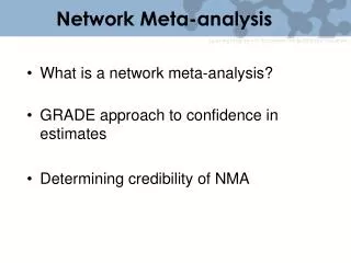
Network Meta-Analysis(Multiple Treatments Meta-Analysis, Mixed Treatment Comparisons) • Combine direct + indirect estimates of multiple treatment effects • Internally consistent set of estimates that respects randomization • Estimate effect of each intervention relative to every other whether or not there is direct comparison in studies • Calculate probability that each treatment is most effective • Compared to conventional pair-wise meta-analysis: • Greater precision in summary estimates • Ranking of treatments according to effectiveness 17
Single Contrast Distributions of observations Distribution of random effects C A
Closed Loop of Contrasts Distribution of random effects Distributions of observations C A B Functional parameter mBC expressed in terms of basic parameters mAB and mAC
Closed Loop of Contrasts Distribution of random effects Distributions of observations C Three-arm study A B
Measuring Inconsistency Suppose we have AB, AC, BC direct evidence Indirect estimate Measure of inconsistency: Approximate test (normal distribution): with variance 23
Basic Assumptions • Transitivity (Similarity) • Trials involving treatments needed to make indirect comparisons are comparable so that it makes sense to combine them • Needed for valid indirect comparison estimates • Consistency • Direct and indirect estimates give same answer • Needed for valid mixed treatment comparison estimates
Five Interpretations of Transitivity Salanti (2012) Treatment C is similar when it appears in AC and BC trials ‘Missing’ treatment in each trial is missing at random There are no differences between observed and unobserved relative effects of AC and BC beyond what can be explained by heterogeneity The two sets of trials AC and BC do not differ with respect to the distribution of effect modifiers Participants included in the network could in principle be randomized to any of the three treatments A, B, C.
Inconsistency vs. Heterogeneity • Heterogeneity occurs within treatment comparisons • Type of interaction (treatment effects vary by study characteristics) • Inconsistency occurs across treatment comparisons • Interaction with study design (e.g. 3-arm vs. 2-arm) or within loops • Consistency can be checked by model extensions when direct and indirect evidence is available
Multinomial Network Example Population: Patients with cardiovascular disease Treatments: High and Low statins, usual care or placebo Outcomes: Fatal coronary heart disease (CHD) Fatal stroke Other fatal cardiovascular disease (CVD) Death from all other causes Non-fatal myocardial infarction (MI) Non-fatal stroke No event Design: RCTs
Multinomial Network 4 studies High Dose Statins Low Dose Statins 9 studies 4 studies Control
Subset of Example • 3 treatments • 3 outcomes
Multinomial Model For each treatment arm in each study, outcome counts follow multinomial distributions Studies k = 1, 2, …, I, Treatments j = 0, 2, …, J-1 Outcomes m = 0, 2, …, M-1
Baseline Category Logits Model k study m outcome j treatment • Multinomial probabilities are re-expressed relative to reference • Model as function of study effect and treatment effect Treatment effects are set of basic parameters representing random effects for txj relative to tx 0 in study k for outcome m • Study effects may apply to different “base” tx in each study • Random treatment effects centered around fixed “d’s”
Random Effects Model Combine across outcomes: so that
Random Effects Model for Tx Effects Σij is covariance matrix between treatments i and j among different outcome categories with djm is average treatment effect for outcome m and treatment j relative to reference treatment 0
Homogeneous Variance Covariance between arms that share treatment Covariance between arms that do not share treatment
Incomplete Treatments • Usual assumption that treatments ordered so that lowest numbered is base treatment b(k) in study k for b < j; j = 1, …, J; m = 1, …, M are fixed effects
Incomplete Treatments Collecting treatments together
Prior Distributions Noninformative normal priors for means dj = (dj1, dj2, …, djM-1) ~ NM-1(0,106 xIM-1) • Implies that event probabilities in no event reference group are centered at 0.5 with standard deviation of 2 on logit scale • This implies that event probabilities lie between 0.02 and 0.98 with probability 0.95, sufficiently broad to encompass all reasonable results
Noninformative Inverse Wishart Priors Σ~ InvWish(R,ν) • R is the scale factor, ν is the degrees of freedom • Minimum value of ν is rank of covariance matrix • R may be interpreted as an estimate of the covariance matrix • Choosing R as the identity matrix implies that the prior standard deviations and variances are each one on the log scale • A 95% CI is then approximately log OR +/- 2 which corresponds to a range for the OR of about [1/7, 7]
Noninformative Inverse Wishart Priors • As R→0, posterior approaches likelihood • Implies very small prior covariance matrix and runs into same problems as inverse gamma prior with small parameters • Too much weight is placed on small variances and so prior is not really noninformative • Study effects are shrunk toward their mean • Could instead choose R with reasonable diagonal elements that match reasonable standard deviation • Still assumes independence • One degree of freedom parameter which implies same amount of prior information about all variance parameters
Variance Structure Factor covariance matrix Σ= SRS where S is diagonal matrix of standard deviations R is correlation matrix Then factor Σ as f(Σ) = f(S)f(R|S) • More information about standard deviations and correlations • Lu and Ades (2009) have implemented this for MTM
Data Setup • Each study has 7 possible outcomes and 3 possible treatments • Not all treatments carried out in each study • Not all outcomes observed in each study • Incomplete data with partial information from summary categories • Can use available information to impute missing values • Can build this into Bayesian algorithm
Missing Data Parameters • Treat missing cell values as unknown parameters • Need to account for partial sums known (e.g. all deaths, all FCVD, all stroke) • May be able to treat sum of two categories as single category • Can use multiple imputation to fill in missing data and then perform complete data analysis • Can incorporate uncertainty of missing cells into probability model
Imputations for Missing Data via MCMC • EM gives us ‘‘plug-in’’ expected values for whatever we are treating as missing data • MCMC gives us a sample of ‘‘plug-in’’ values --- or multiple imputations • MCMC allows averaging over uncertainty in model’s other random quantities when making inferences about any particular random quantity (either missing data point or parameter) • Bottom line: really no distinction between missing data point and parameter
Example of Imputation Imputing FS in IDEAL trial: • Bounded by 48 (total of FS + OFCVD) • Ratio of FS/(FS+OFCVD) between 0.14 and 0.69 with median about 0.5 • Logical choice is Bin (48, p) where p is probability of FS as fraction of all strokes • Choose beta prior on p that fits data range, say beta(6,6)