TECHNIQUES ALGORITHMS AND SOFTWARE FOR THE DIRECT SOLUTION OF LARGE SPARSE LINEAR EQUATIONS
500 likes | 602 Vues
TECHNIQUES ALGORITHMS AND SOFTWARE FOR THE DIRECT SOLUTION OF LARGE SPARSE LINEAR EQUATIONS. Wish to solve Ax = b A is LARGE and S P A R S E. A LARGE . . . ORDER n(t) t n 1970 200 1975 1 000 1980 10 000

TECHNIQUES ALGORITHMS AND SOFTWARE FOR THE DIRECT SOLUTION OF LARGE SPARSE LINEAR EQUATIONS
E N D
Presentation Transcript
TECHNIQUES ALGORITHMS AND SOFTWARE FOR THE DIRECT SOLUTION OF LARGE SPARSE LINEAR EQUATIONS
Wish to solve Ax = b A is LARGE and S P A R S E
A LARGE . . . ORDER n(t) t n 1970 200 1975 1 000 1980 10 000 1985 100 000 1990 250 000 1995 500 000 2000 2 000 000 SPARSE . . . NUMBER ENTRIES kn k ~ 2 - log n
NUMERICAL APPLICATIONS Stiff ODEs … BDF … Sparse Jacobian Linear Programming … Simplex Optimization/Nonlinear Equations Elliptic Partial Differential Equations Eigensystem Solution Two Point Boundary Value Problems Least Squares Calculations
APPLICATION AREAS Physics CFD Lattice gauge Atomic spectra Chemistry Quantum chemistry Chemical engineering Civil Engineering Structural analysis Electrical Engineering Power systems Circuit simulation Device simulation Geography Geodesy Demography Migration Economics Economic modelling Behavioural sciences Industrial relations Politics Trading Psychology Social dominance Business administration Bureaucracy Operations research Linear Programming
THERE FOLLOWS PICTURES OF SPARSE MATRICES FROM VARIOUS APPLICATIONS This is done to illustrate different structures for sparse matrices
STANDARD SETS OF SPARSE MATRICES Original set Harwell-Boeing Sparse Matrix Collection Available by anonymous ftp from: ftp.numerical.rl.ac.uk or from the Web page: http://www.cse.clrc.ac.uk/Activity/SparseMatrices Extended set of test matrices available from: Tim Davis http://www.cise.ufl.edu/research/sparse/matrices
RUTHERFORD-BOEING SPARSE MATRIX TEST COLLECTION • Unassembled finite-element matrices • Least-squares problems • Unsymmetric eigenproblems • Large unsymmetric matrices • Very large symmetric matrices • Singular Systems • See Report: • The Rutherford-Boeing Sparse Matrix Collection • Iain S Duff, Roger G Grimes and John G Lewis • Report RAL-TR-97-031, Rutherford Appleton Laboratory • http://www.numerical.rl.ac.uk/reports/reports • To be distributed via matrix market • http://math.nist.gov/MatrixMarket
RUTHERFORD - BOEING SPARSE MATRIX COLLECTION Anonymous FTP to FTP.CERFACS.FR cd pub/algo/matrices/rutherford_boeing OR http://www.cerfacs.fr/algor/Softs/index.html
notation only. Do not use or even think of inverse of A. For Sparse A, A-1 is usually dense [eg A tridiagonal arrowhead ] A x = b has solution x = A-1b
DIRECT METHODS Gaussian Elimination PAQ LU Permutations P and Q chosen to preserve sparsity and maintain stability L : Lower triangular (sparse) U : Upper triangular (sparse) SOLVE: Ax = b by Ly = Pb then UQx = y
PHASES OF SPARSE DIRECT SOLUTION • Although the exact subdivision of tasks for sparse direct solution will depend on the algorithm and software being used, a common subdivision is given by: • ANALYSE An analysis phase where the matrix • is analysed to produce a suitable ordering and • data structures for efficient factorization. • FACTORIZE A factorization phase where the • numerical factorization is performed. • SOLVE A solve phase where the factors are used to • solve the system using forward and backward • substitution. • We note the following: • ANALYSE is sometimes preceded by a • preordering phase to exploit structure. • For general unsymmetric systems, the ANALYSE • and FACTORIZE phases are sometimes combined • to ensure the ordering does not compromise • stability. • Note that the concept of separate FACTORIZE • and ANALYSE phases is not present for dense • systems.
STEPS MATCH SOLUTION REQUIREMENTS 1. One-off solution Ax = b A/F/S 2. Sequence of solutions [Matrix changes but structure is invarient] A1x1 = b1 A2x2 = b2 A/F/S/F/S/F/S A3x3 = b3 3. Sequence of solutions [Same matrix] Ax1 = b1 Ax2 = b2 A/F/S/S/S Ax3 = b3 For example …. 2. Solution of nonlinear system A is Jacobian 3. Inverse iteration
TIMES (MA48) FOR ‘TYPICAL’ EXAMPLE [Seconds on CRAY YMP … matrix GRE 1107] ANALYSE/FACTORIZE .66 FACTORIZE .075 SOLVE .0068
DIRECT METHODS • Easy to package • High accuracy • Method of choice in many applications • Not dramatically affected by • conditioning • Reasonably independent of structure • However • High time and storage requirement • Typically limited to n ~ 1000000 • So • Use on subproblem • Use as preconditioner
COMBINING DIRECT AND ITERATIVE METHODS … can be thought of as sophisticated preconditioning. Multigrid … using direct method as coarse grid solver. Domain Decomposition … using direct method on local subdomains and ‘direct’ preconditioner on interface. Block Iterative Methods … direct solver on sub-blocks Partial Factorization as Preconditioner ‘Full’ Factorization of Nearby Problem as a Preconditioner.
FOR EFFICIENT SOLUTION OF SPARSE EQUATIONS WE MUST • Only store nonzeros (or exceptionally a • few zeros also) • Only perform arithmetic with nonzeros • Preserve sparsity during computation
COMPLEXITY of LU factorization on dense matrices of order n 2/3 n3 + 0(n2) flops n2 storage For band (order n, bandwidth k) 2 k2n work, nk storage Five-diagonal matrix (on k x k grid) 0 (k3) work and 0 (k2 log k) storage Tridiagonal + Arrowhead matrix 0 (n) work + storage Target 0 (n) + 0 () for sparse matrix of order n with entries
x 6 x x x x x 4 5 1 2 6 GRAPH THEORY We form a graph on n vertices associated with our matrix of order n. Edge (i, j) exists in the graph if and only if entry aij (and, by symmetry aji) in the matrix is non-zero. Example x x x x x x x x x x x x x x Symmetric Matrix and Associated Graph
MAIN BENEFITS OF USING GRAPH THEORY IN STUDY OF SYMMETRIC GAUSSIAN ELIMINATION 1. Structure of graph is invariant under symmetric permutations of the matrix (corresponds to re- labelling of vertices). 2. For mesh problems, there is usually an equivalence between the mesh and the graph associated with the resulting matrix. We thus work directly with the underlying structure. 3. We can represent cliques in graphs by listing vertices in a clique without storing all the interconnecting edges.
COMPLEXITY FOR MODEL PROBLEM Model Problem with n variables Ordering Time 0 (1) .. 0 (n) Symbolic 0 (n) Factorization Numerical 0 (n3/2) Solve 0 (n log2 n) and big 0 is not so big
Ordering for sparsity … unsymmetric matrices *x x x v v x v v x v v ri = 3, cj = 4 Minimize (ri - 1) * (cj - 1) MARKOWITZ ORDERING (Markowitz 1957) Choose nonzero satisfying numerical criterion with best Markowitz count
Benefits of Sparsity on Matrix of Order 2021 with 7353 entries Total Storage Flops Time (secs) Procedure (Kwords) (106) CRAY J90 Treating system as dense 4084 5503 34.5 Storing and operating 71 1073 3.4 only on nonzero entries Using sparsity pivoting 14 42 0.9
An example of a code that uses Markowitz and Threshold Pivoting is the HSL Code MA48
Comparison between sparse (MA48 from HSL) and dense (SGESV from LAPACK). Times for factorization/solution in seconds on CRAY Y-MP.
HARWELL SUBROUTINE LIBRARY • Started at Harwell in 1963 • Most routines from research work of group • Particular strengths in: • - Sparse Matrices • - Optimization • - Large-Scale system solution • Since 1990 Collaboration between RAL and • Harwell • HSL 2000 . . . October 2000 • URL: http://www.cse.clrc.ac.uk/Activity/HSL
Wide Range of Sparse Direct Software • Markowitz + Threshold MA48 • Band - Variable Band (Skyline) MA55 • Frontal • - Symmetric MA62 • - Unsymmetric MA42 • Multifrontal • - Symmetric MA57 and MA67 • - Unsymmetric MA41 • - Very Unsymmetric MA38 • - Unsymmetric element MA46 • Supernodal SUPERLU
Features of MA48 • Uses Markowitz with threshold privoting • Factorizes rectangular and singular systems • Block Triangularization • - Done at ‘higher’ level • - Internal routines work only on single • block • Switch to full code at all phases of solution • Three factorize entries • - Only pivot order is input • - Fast factorize .. Uses structures generated • in first factorize • - Only factorizes later columns of matrix • Iterative refinement and error estimator in • Solve phase • Can employ drop tolerance • ‘Low’ storage in analysis phase
TWO PROBLEMS WITH MARKOWITZ & THRESHOLD 1. Code Complexity Implementation Efficiency 2. Exploitation of Parallelism
TYPICAL INNERMOST LOOP DO 590 JJ = J1, J2 * J = ICN (JJ) IF (IQ(J). GT.0) GO TO 590 IOP = IOP + 1 * PIVROW = IJPOS - IQ (J) A(JJ) = A(JJ) + AU x A (PIVROW) IF (LBIG) BIG = DMAXI (DABS(A(JJ)), BIG) IF (DABS (A(JJ)). LT. TOL) IDROP = IDROP + 1 ICN (PIVROW) = ICN (PIVROW) 590 CONTINUE
INDIRECT ADDRESSING • Increases memory traffic • Results in bad data distribution and non- • localization of data • And non-regularity of access • Suffers from short ‘vector’ lengths
SOLUTION Isolate indirect addressing W(IND(I)) from inner loops(s). Use full/dense matrix kernels (Level 2 & 3 BLAS) in innermost loops.
MAIN PROBLEM WITH PARALLEL IMPLEMENTATION IS THAT SPARSE DIRECT TECHNIQUES 1. REDUCE GRANULARITY 2. INCREASE SYNCHRONIZATION 3. INCREASE FRAGMENTATION OF DATA
PARALLEL IMPLEMENTATION X X X X X X Obtain by choosing entries so that no two lie in same row or column. Then do rank k update.
TECHNIQUES FOR USING LEVEL 3 DENSE BLAS IN SPARSE FACTORIZATION Frontal methods (1971) Multifrontal methods (1982) Supernodal methods (1985) All pre-dated BLAS in 1990
BLAST BLAS TECHNICAL FORUM Web Page: www.netlib.org/blas/blast-forum has both: Dense and Sparse BLAS