Section 6.3
Understand and calculate confidence intervals for the difference between two population means using equal variance assumptions, with step-by-step instructions for Excel. Includes relevant formulas and definitions.

Section 6.3
E N D
Presentation Transcript
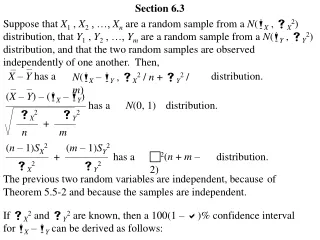
Section 6.3 Suppose that X1 , X2 , …, Xn are a random sample from a N(X , X2) distribution, that Y1 , Y2 , …, Ym are a random sample from a N(Y , Y2) distribution, and that the two random samples are observed independently of one another. Then, N(X– Y, X2 / n + Y2 / m) X– Y has a distribution. (X–Y) – (X– Y) ———————– has a distribution. X2Y2 —— + —— nm N(0, 1) (n – 1)SX2 (m – 1)SY2 ———— + ———— has a distribution. X2Y2 2(n + m –2) The previous two random variables are independent, because If X2 and Y2 are known, then a 100(1 – )% confidence interval for X– Y can be derived as follows: of Theorem 5.5-2 and because the samples are independent.
(X–Y) – (X– Y) – z/2 ———————– z/2 = 1 – 2X2Y —— + —— nm P – (X–Y) – z/2 2X / n + 2Y / m P – (X– Y) = 1 – – (X–Y) + z/2 2X / n + 2Y / m (X–Y) – z/2 2X / n + 2Y / m P X– Y = 1 – (X–Y) + z/2 2X / n + 2Y / m Note: If X2 and Y2 are not known, then for a sufficiently large sample size, we can still use this confidence interval by respectively substituting sX2 and sY2 in place of X2 and Y2 .
If X2 = Y2 = 2 , but 2 is not known, then (X–Y) – (X– Y) ———————– X2Y2 — + — nm = (n – 1)SX2+ (m – 1)SY2 ———— ———— X2 Y2 n + m –2 = (X–Y) – (X– Y) ———————– 1 1 — + — nm (n – 1)SX2+ (m – 1)SY2 1 — n + m –2
(X–Y) – (X– Y) —————————————— (n – 1)SX2 + (m – 1)SY2 1 1 ————————— — + — n + m – 2 nm has a distribution. t(n + m –2) If X2 = Y2 = 2 , but 2 is not known, then a 100(1 – )% confidence interval for X– Y can be derived as follows: (X–Y) – (X– Y) —————————————— (n – 1)SX2 + (m – 1)SY2 1 1 ————————— — + — n + m –2 nm P – t/2(n + m –2) t/2(n + m –2) = 1 –
(X–Y) – (X– Y) —————————————— (n – 1)SX2 + (m – 1)SY2 1 1 ————————— — + — n + m –2 nm P – t/2(n + m –2) t/2(n + m –2) = 1 – P (X–Y) – t/2(n + m –2) Sp1/n + 1/m X– Y (X–Y) + t/2(n + m –2) Sp1/n + 1/m = 1 – (n – 1)SX2 + (m – 1)SY2 ————————– n + m –2 where Sp2 = is called the pooled sample variance.
Note: If the random sample does not come from a normal distribution, then for sufficiently large sample sizes we can still use these confidence intervals, which are listed in the summary displayed on the back page of the text. If X2 and Y2 are not known, and it cannot be assumed they are equal, then an approximate 100(1 – )% confidence interval for X– Y can be obtained from Welch’s derivation outlined at the end of Section 6.3 in the text.
1. Do Text Exercise 6.3-1. (937.4 – 988.9) 1.645784 / 56 + 627 / 57 The 90% confidence interval for X– Y is – 59.725 < X– Y < – 43.275 We are 90% confident that mean length of life of brand X bulbs is between 43.275 and 59.725 hours smaller than the mean length of life of brand Y bulbs.
2. (a) (1) (2) (3) (4) Add a worksheet to the Excel file Confidence_Intervals (created in Class Exercise #4 in Section 6.2) which displays the limits of a confidence interval for the difference between two means, assuming equal variance and based on the Student’s t distribution. Create a worksheet named Two Sample in the Excel file named Confidence_Intervals as follows: In Sheet2, select cells A1:B500, and color these cells with a light color such as yellow. Change the name of Sheet2 to Two Sample. Color the cell F9 with a light color such as yellow. Enter the labels displayed in columns C through H, and right justify the labels in columns E and H.
(5) (6) Select cells A1:A500. From the main menu, select the Formulas tab, select the option Name Manager, and click the New button in the dialog box which appears. (7) Type the new range name Data1, and click the OK button to return to the Name Manager dialog box. (8) With the Name Manager dialog box still open, click the New button, type the new range name Data2, and click inside the Refers to slot. (9) With the Refers to slot selected, select cells B1:B500, click the OK button to return to the Name Manager dialog box, and click the Close button to close the dialog box. (10) Select cells E1:F4, and in the Formulas tab select the option Create from Selection; then, with Left column checked in the dialog box that appears, click OK. (11) Select cells H1:I4, and in the Formulas tab select the option Create from Selection; then, with Left column checked in the dialog box that appears, click OK. (12) Select cells F6:G6, and in the Formulas tab select the option Create from Selection; then, with Left column checked in the dialog box that appears, click OK. (13) Enter the following formulas respectively in cells F1:F4: =COUNT(Data1) =IF(COUNT(Data1)>0,AVERAGE(Data1),"-") =IF(COUNT(Data1)>1,VAR(Data1),"-") =IF(COUNT(Data1)>1,STDEV(Data1),"-")
2.-continued (14) Enter the following formulas respectively in cells I1:I4: =COUNT(Data2) =IF(COUNT(Data2)>0,AVERAGE(Data2),"-") =IF(COUNT(Data2)>1,VAR(Data2),"-") =IF(COUNT(Data2)>1,STDEV(Data2),"-") (15) Enter the following formula in cell G6: =IF(AND(n_1>0,n_2>0),((n_1-1)*Variance_1+(n_2-1)*Variance_2)/(n_1+n_2-2),"-") (16) Enter the following formulas respectively in cells F10:F12: =IF(AND(n_1>0,n_2>0,$F$9>0,$F$9<1),TINV(1-$F$9,n_1+n_2-2),"-") =IF(AND(n_1>0,n_2>0,$F$9>0,$F$9<1), Mean_1-Mean_2-$F$10*SQRT(Pooled_Sample_Variance*(1/n_1+1/n_2)),"-") =IF(AND(n_1>0,n_2>0,$F$9>0,$F$9<1), Mean_1-Mean_2+$F$10*SQRT(Pooled_Sample_Variance*(1/n_1+1/n_2)),"-") (17) Save the file as Confidence_Intervals (in your personal folder on the college network).
(b) Use the Excel file Confidence_Intervals to obtain a two-sided confidence interval in Text Exercise 6.3-5. (Open Excel file Data_for_Students in order to copy the data of Exercise 6.3-5.) Suppose we assume the variances are equal. We are 95% confident that mean length of a male green lynx spider is between 1.740 and 2.734 millimeters smaller than the mean length of a female green lynx spider. 3. Use the Excel file Confidence_Intervals to obtain the confidence interval in Text Example 6.3-4. (Open Excel file Data_for_Students in order to copy the data of Example 6.3-4.) Since this is paired data (i.e. not independent samples!), we need a one sample confidence interval for the mean difference (instead of a two sample confidence interval for the difference between means). The 95% confidence interval for the mean difference contains zero (0), which implies that there is no statistically significant difference in mean reaction time to red lights and green lights.