Download
1 / 64
690 likes | 1.06k Vues
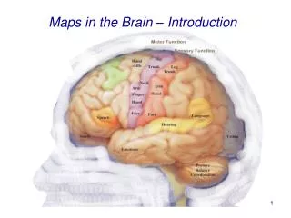
Maps in the Brain – Introduction. Overview. A few words about Maps Cortical Maps: Development and (Re-)Structuring Auditory Maps Visual Maps Place Fields. What are Maps I. Intuitive Definition: Maps are a (scaled) depiction of a certain area.

E N D
Overview A few words about Maps Cortical Maps: Development and (Re-)Structuring Auditory Maps Visual Maps Place Fields
What are Maps I Intuitive Definition: Maps are a (scaled) depiction of a certain area. Location (x,y) is directly mapped to a piece of paper. Additional information such as topographical, geographical, political can be added as colors or symbols.
What are Maps I Intuitive Definition: Maps are a (scaled) depiction of a certain area. Location (x,y) is directly mapped to a piece of paper. Additional information such as topographical, geographical, political can be added as colors or symbols. Important: A map is always a reduction in complexity. It is a REDUCED picture of reality that contains IMPORTANT aspects of it. What is important? That is in the eye of the beholder...
What are Maps II Mathematical Definition: Let W be a set, U a subset of W and A metric space (distances are defined). Then we call f a map if it is a one-to-one mapping from U to A. f: U -> A Example: The surface of the world (W) is a 2D structure embedded in 3D space. It can be mapped to a 2D euclidean space. In a mathematical sense a map is an equivalent representation of a complex structure (W) in a metric space (A), i.e. it is not a reduction – the entire information is preserved.
Cortical Maps Cortical Maps map the environment onto the brain. This includes sensory input as well as motor and mental activity. Example: Map of sensory and motor representations of the body (homunculus).The more important a region, the bigger its map representation. Scaled “remapping” to real space
Place Cells Spatial Maps
What are place cells? • Place cells are the principal neurons found in a special area of the mammal brain, the hippocampus. • They fire strongly when an animal (a rat) is in a specific location of an environment. • Place cells were first described in 1971 by O'Keefe and Dostrovsky during experiments with rats. • View sensitive cells have been found in monkeys (Araujo et al, 2001) and humans (Ekstrom et al, 2003) that may be related to the place cells of rats.
The Hippocampus Human hippocampus
The Hippocampus Human hippocampus Rat hippocampus
Place cells Visual Olfactory Auditory Taste Somatosensory Self-motion Hippocampus • Hippocampus involved in learning and memory • All sensory input into hippocampus • Place cells in hippocampus get all sensory information • Information processing via trisynaptic loop • How place are exactly used for navigation is unknown
Place cell recordings 1. • Electrode array is inserted to the brain for simultaneous recording of several neurons. Wilson and McNaughton, 1993
Place cell recordings 1. 2. • Electrode array is inserted to the brain for simultaneous recording of several neurons. • The rat moves around in a known/unknown environment. Wilson and McNaughton, 1993
Place cell recordings 1. 2. • Electrode array is inserted to the brain for simultaneous recording of several neurons. • The rat moves around in a known/unknown environment. • Walking path and firing activity (cyan dots). 3. Wilson and McNaughton, 1993
y y x x Place Field Recordings Terrain: 40x40cm Single cell firing activity • Map firing activity to position within terrain • Place cell is only firing around a certain position (red area) • Cell is like a “Position Detector”
Place fields 40x40cm • Array of cells • Ordered for position of activity peak (top left to bottom right) O’Keefe, 1999
Place fields 40x40cm • Array of cells • Ordered for position of activity peak (top left to bottom right) • Different shapes: • Circular Islands O’Keefe, 1999
Place fields 40x40cm • Array of cells • Ordered for position of activity peak (top left to bottom right) • Different shapes: • Circular Islands • Twin Peaks O’Keefe, 1999
Place fields 40x40cm • Array of cells • Ordered for position of activity peak (top left to bottom right) • Different shapes: • Circular Islands • Twin Peaks • Elongated O’Keefe, 1999
Place fields 40x40cm • Array of cells • Ordered for position of activity peak (top left to bottom right) • Different shapes: • Circular Islands • Twin Peaks • Elongated • Not Simple (=> not published) O’Keefe, 1999
How do place cells develop? • Allothetic (external) sensory input • Visual • Olfactory (around 1000 receptors in rat, whereas humans have 350) • Somatosensory (via whiskers) • Auditory (rat range 200Hz-90KHz, human range 16Hz-20KHz) • Idiothetic (internal) sensory input • Self motion (path integration, mostly used then allothetic information is not available) • Not so reliable by itself since no feedback
Importance of visual cues Experiment: Environment with landmark (marked area) => record activity from cell 1 and 2 Observation: Place fields develop Knierim, 1995
Importance of visual cues Experiment: Environment with landmark (marked area) => record activity from cell 1 and 2 Observation: Place fields develop Step 2: Rotate landmark => place fields rotate respectively Conclusion: Visual cues are used for formation of place fields Knierim, 1995
Place Cell Remapping Brown plastic square box and white wooden circle box was used to show place cell remapping phenomena: • Cells 1-5 show increasing divergence between the square and circle box; • Cells 6-10 show differentiation from the beginning; • Some cells chow common representation or do not remap at all (not shown). Wills et al, 2005, Science
Light/Cleaning Dark/Cleaning Importance of olfactory cues Fact: Rats use their urine to mark environment Experiment: Two sets, one in light and one in darkness; remove self-induced olfactory cues and landmarks (S2-S4) Result: Without olfactory cues stable place fields (control S1) change or in darkness even deteriorate. When olfactory cues are allowed again (control S5), place fields reemerge. Save, 2000
Place cell model • Use neuronal network to model formation of place cells
Place cell model • Use neuronal network to model formation of place cells • Input layer for allothetic sensory input depending on position in simulated world • 4 Visual cues (landmarks)
Place cell model • Use neuronal network to model formation of place cells • Input layer for allothetic sensory input depending on position in simulated world • 4 Visual cues (landmarks) • 4 Olfactory cues (environmental)
Place cell model • Use neuronal network to model formation of place cells • Input layer for allothetic sensory input depending on position in simulated world • 4 Visual cues (landmarks) • 4 Olfactory cues (environmental) • Output layer, n x n simulated neurons, each of which is connected to all input neurons (fully connected feed-forward)
Place cell model • Use neuronal network to model formation of place cells • Input layer for allothetic sensory input depending on position in simulated world • 4 Visual cues (landmarks) • 4 Olfactory cues (environmental) • Output layer, nxn simulated neurons, each of which is connected to all input neurons (fully connected feed-forward) • After learning => formation of place fields
Place cell model • Use neuronal network to model formation of place cells • Input layer for allothetic sensory input depending on position in simulated world • 4 Visual cues (landmarks) • 4 Olfactory cues (environmental) • Output layer, nxn simulated neurons, each of which is connected to all input neurons (fully connected feed-forward) • After learning => formation of place fields • The know-how is in the change of the connection weights W ...
Mathematics of the model • Firing rate r of Place Cell i at time t is modeled as Gaussian function: σf is width of the Gaussian function, X and W are vectors of length n, ||* || is theeuclidean distance
Mathematics of the model • Firing rate r of Place Cell i at time t is modeled as Gaussian function: σf is width of the Gaussian function, X and W are vectors of length n, ||* || is theeuclidean distance • At every time step only on weight W is changed (Winner-Takes-All), i.e. the neuron with the strongest response is changed:
Place fields • Visual input => unique round place fields, because the distances to the walls are unique (no multipeaks) • Olfactory input => place fields not round, because input is complex (gradients not well structured) • Combined input is a mixture of both
Cortical Mapping Retinal(x,y) tocomplex log coordinates Retinal SpaceComplex log ConcentricCirclesVertical Lines (expon. Spaced) (equallyspaced) Radial Lines Horizontal Lines (equalangular spacing) (equallyspaced) The complexlogarithmictransform a = c + ib log(a) = log(c + ib) In Polar Coordinates a = r exp(if) b r = ||a|| f c
Cortical Mapping retinal (x,y) to log Z Coordinates On „Invariance“ A majorproblemishowthebraincanrecognizeobject in spiteofsizeandrotationchanges! Real Space log Z Space ConcentricCirclesVertical Lines (expon. Spaced) (equallyspaced) Radial Lines Horizontal Lines (equalangular spacing) (equallyspaced) Scalingand Rotation defined in Polar Coordinates: Scaling A = k r exp(if) = k a a = r exp(if) Scalingconstant Rotation A = exp(ig) r exp(if) = r exp(i[f+g]) = a exp(ig) Rotation angle After log Z transformweget: Scaling: log(ka) = log(k) + log(a) Rotation: log(a exp(ig)) = ig + log(a) Thus wehaveobtainedscaleandrotationinvariance !
Somemoredetails z+a z=x + iy G(z) = log z+b a and b take the values 0.333 and 6.66 respectively.
Visual Cortex Primary visual cortex or striate cortex or V1. Well defined spacial representation of retina (retinotopy).
Visual Cortex Primary visual cortex or striate cortex or V1. Well defined spacial representation of retina (retinotopy). Prestriate visual cortical area or V2 gets strong feedforward connection from V1, but also strongly projects back to V1 (feedback) Extrastriate visual cortical areas V3 – V5. More complex representation of visual stimulus with feedback from other cortical areas (eg. attention).
Receptive fields Cells in the visual cortex have receptive fields (RF). These cells react when a stimulus is presented to a certain area on the retina, i.e. the RF. Simple cells react to an illuminated bar in their RF, but they are sensitive to its orientation (see classical results of Hubel and Wiesel, 1959). Bars of different length are presented with the RF of a simple cell for a certain time (black bar on top). The cell's response is sensitive to the orientation of the bar.
On-Off responses Experiment: A light bar is flashed within the RF of a simple cell in V1 that is recorded from. Observation: Depending on the position of the bar within the RF the cell responds strongly (ON response) or not at all (OFF response).