Scanning Probe Microscopy for Complex Materials
University of Pune. Scanning Probe Microscopy for Complex Materials. Prof. C. V. Dharmadhikari Center for Advanced Studies in Materials Science and Condensed Matter Department of Physics. Scanning Tunneling Microscopy: Principle. Expression for tunneling current.

Scanning Probe Microscopy for Complex Materials
E N D
Presentation Transcript
University of Pune Scanning Probe Microscopy for Complex Materials Prof. C. V. Dharmadhikari Center for Advanced Studies in Materials Science and Condensed Matter Department of Physics
Expression for tunneling current I V s (0,EF) e-2kz Where I = tunneling current flowing between tip and sample V = Applied bias voltage s= Density of states of sample k = Decay constant which depends on the average work functions of tip and sample z = Distance between tip sample
The tunneling current depends exponentially on the distance between • The tip and the sample. • Thus when the tip is scanned over the sample the topographic • information can be obtained by grabbing the change in the tunneling • current. • The tip sample junction stability and the sharpness of the tip are • the important criteria which decides the resolution of the • instrument SEM picture of the STM tip which is Used for imaging
STM is operated in two modes: 1. Constant current mode 2. Constant distance mode Scanning Tunneling Spectroscopy (STS) I V s (0,EF) e-2kz • If the distance between the tip and sample is kept constant and the • applied bias is varied the change is tunneling current with bias gives • the information about the local density of states of the sample.
Conductance spectra of electrodeposited CdSe nanocrystal at various tip-sample • Distances (b) Conductance spectra for covalently anchored colloidal nanocrystal P. Erik et.al. Phys. Rev. B, 62, R7743 (2000)
Electron transport study of nanostructures using Scanning Probe Microscopy • Electron transfer mechanism in nanoparticles can be studied using STM tip. • Double barrier tunnel junction (DBTJ) is formed between the tip-nanoparticle and nanoparticle-substrate junction. Electronic properties of individual nanoparticles can be studied using tunneling spectroscopy. Schematic representation of substrate/nanoparticle/tip junction
When a small bias is applied to the tip the resonant tunneling of electron from tip to dot and dot to substrate occurs when Ef tip reaches the first discrete conduction band level of the nanoparticle. • Zero current in the I-V curve represents the gap of the nanoparticle and steps represent the discrete energy levels of nanoparticle. In this way size dependent properties of nanostructures can be probed using Scanning Tunneling Spectroscopy (STS)
Schematic of electrodeposited nanocrystal on the substrate, • (b) Covalent anchoring of colloidal nanocrystal P. Erik et. al. Phys. Rev. B, 62, R7743 (2000)
Coulomb Blockade effect In addition to size dependent modification of band structure strong capacitance is associated with nanostructure which affects the electronic structure giving rise to single electron charging effects reflected as coulomb blockade, staircase features in current-voltage plots Schematic representation of DBTJ with STM tip, nanoparticle and substrate. Electrical equivalent circuit of DBTJ.
Orthodox theory The average current is given by: Where, r1(N,V) and l1(N,V) are the electron tunneling rates from the right and left, respectively on the first junction. (N, V, t) is the probability that there are N extra electrons on the middle electrode at time t with applied voltage V. From Fermi Golden rule calculation tunneling rate is given by: M.Amman and R.Wilkins, PRB, 43,1146,(1991)
Assuming Dr (E), Dm (E) and |T(E)2| to be energy independent so Dr (E)=Dr0, Dm (E)=Dm0 and |T(E)2| = |T02| Where R1= ħ/(2e2Dr0Dm0 |T02| is the normal state resistance of first junction and E r-E m is the energy the electron gains during the tunneling event. If it is assumed that the charge distribution completely relaxes during the tunneling event, the energy difference is given by: Junction Charging energy M.Amman and R.Wilkins, PRB, 43,1146,(1991)
The resultant tunneling rate turns out to be: • In the above equation its clear that at T = 0 K tunneling is suppressed • for eV1< Ec where Ecis the charging energy of the junction. These two equation can be solved by numerical methods to calculate the I-V characteristics. M.Amman and R.Wilkins, PRB, 43,1146,(1991)
I-V Characteristics • Conductance spectra of electrodeposited CdSe nanocrystal at various tip-sample distances. • Conductance spectra for covalently anchored colloidal nanocrystal P. Erik et.al. Phys. Rev. B, 62, R7743 (2000)
For Coulomb blockade phenomena, Charging energy of nanoparticle should satisfy two conditions: 1. Ec= e2/2C >> KBT 2. Ec>> h/T Where T = RTC is the single electron tunneling time and RTis the tunnel resistance. Thus RT >> RQ h/e2 = 26 k This condition ensures that electrons are tunneling the insulating gap one at a time.
Schematic energy level diagram showing Coulomb blockade in nanocrystal system In order to add or remove one electron from or to the nanocrystal the Fermi energy of the sample must be raised. Thus, there will be a range of bias voltage for which there wont be any onductance which will be seen in The I-V characteristics of the nanocluster.
InAs Radojkovic et al. J. Vac. Sci. Technol. B, 14, No. 2, (1996) U. Banin et.al, Nature, 400, 542 (1999)
STM study of Dodecane Thiol (DDT) capped Au nanopartilces deposited on HOPG N. K. Chaki, P. Singh, C. V. Dharmadhikari and K.P.Vijayamohanan,Langmuir,20 (23),10208 (2004) DDT- C12H25SH Chain lenghth-1.5nm
Theory Experimental Ec Experimental I-V fitted with Theoretical I-V N. K. Chaki, P. Singh, C. V. Dharmadhikari and K.P.Vijayamohanan,Langmuir,20(23),10208 (2004)
Best Fit parameters obtained after fitting are: R1= 108 ohms , C1= 1 x 10 -19 F R2= 106 ohms, C2= 2.5 x 10 -20 F Cg1 = 2.8 x 10 -19 F, Vg1= 0 V Cg2= 0 F, Vg2= 0 V, Q0= 0 Vb = 0.l7 V, Ec= 0.19 eV, kT/Ec=0.1307 and T =300K Using simple Spherical model Capacitance C= 40rr = 7.495 x 10 -19 F , where r= 3 (for DDT), r ~ 2.25 nm 0=8.85 x 10⁻¹²F/m Ec= e2/2C = 0.106 eV Variation in the value of Ec: (1) Simple orthodox model is inadequate in this region (2) Model based on electron transport in MIM is required to understand the electron transport in present case. Inspite of these deviation STM/STS studies show that these larger particles are accessible for single electron charging in air despite their higher capacitance values.
Scan Area : 300 x 300 Å STM image of Dodecane Thiol (DDT) capped Au nanopartilces deposited on HOPG Line profile showing particle size ≈ 4 nm DDT- C12H25SH Chain lenghth-1.5nm N.K.Chaki, B.Kakade, K.P.Vijayamohanan, P.Singh and C.V,Dharmadhikari: Phys. Chem. Phys. (Germany) 8, 1 (2006)
(b) (a) Current (nA) Bias(V) Experimental I-V fitted with Theoretical I-V Based on orthodox model Experimental Theory
Best fit parameters for the offset corrected I-V data that results into good fit with the theoretical curve are: R1= 108 ohms , C1= 5 x 10-20 F R2 = 106 ohms, C2= 7 x 10-19 F Cg1 = 1 x 10-22 F, Vg1= 0 V Cg2= 0 F, Vg2= 0 V, Q0(e)= -0.05 Vb = 0.l5 V, Ec= 0.11 eV, kT/Ec=0.242 and T =300 K Using simple Spherical model : Capacitance C= 40rr = 6.67 x 10⁻¹⁹ F , where r= 3 (for DDT), r ~ 2 nm 0=8.85 x 10⁻¹²F/m Ec= e2/2C = 0.12 eV STM/STS studies show that these larger particles are accessible for single electron charging in air despite their higher capacitance values.
Scanning Tunneling Microscopy and Spectroscopy studies on isolated TiO2nanoparticle Suwarna et.al., Colloids and Surfaces A, 232/1, 11 (2003)
Analysis • The image clearly shows the isolated nanoparticles. IV was performed • on single nanoparticle. dI/dV mimics the local density of states of the • surface. • The two prominent peaks in the dI/dV curve at 0.7 eV and 1.4 eV are • consistent with the theoretical calculation for defect induced state and • for OH- - (TiO4)n- cluster. • The observed band gap of around 3 eV is comparable to the bulk band • gap of TiO2. • For the interpretation of spectroscopy result it is important to • consider the distribution of bias voltage over substrate-nanoparticle • and nanoparticle-tip junction • By varying the size of the nanoparticle one can systematically observe • the size dependent changes in the electronic structure of the isolated • nanoparticle.
STM studies of Au nanoparticles functionalised with organic legands Au nanoparticles functionalized with Lauryl Amine (R-NH2,R= 12 C atoms, length 1.7 nm(50 x 50 nm) Suwarna Datar, PhD Thesis 2004
Cotnd…. Au nanoparticles functionalized with Octadecane thiol (R-SH, R= 18 C atoms, Length 2.7 nm) (50 x 50 nm) Suwarna Datar, PhD Thesis 2004
(a) (b) (c) (d) FIG.1.(a) Constant current STM image of HOPG surface (Scan area: 20 x 20 Å2,I = 1.14 nA, V = - 0.023 V) (b) STM image of agglomeration of nanoclusters deposited on HOPG (Scan area: 1500 x 1500 Å2, I = 0.5 nA, V = 0.47 V). (c) STM image of nanoparticles at the step edge deposited on HOPG (Scan area: 380 x 530 Å2, I=0.5nA, V=0.47 V). (d) Line profile of the nanoparticles shown in (b). Electron Transport on DDT-capped Au nanoparticles on HOPG- I-S measurements
Plot of ln I (I in Amperes) versus distance “s” (s in Angstroms) on agglomeration of nanoclusters (marked by ‘o’) and on isolated nanocluster (marked by ‘Δ’). Left inset shows the plot of ln I (I in Amperes) versus distance “s” (s in Angströms) for bare HOPG (marked by ‘o’) and nanocluster at the step edge (marked by ‘Δ’) to calculate the barrier height at different sites. Right inset shows I-V taken on bare HOPG. ln I ln I Distance (Å) Distance (Å) Contd..
Contd.. I-V taken on isolated nano (marked by ‘o’). Left inset shows I-V taken on nanocluster at the step edge (marked by ‘o’). Right inset shows the I-V taken on array of nanocluster (marked by ‘o’). Each curve is an average of eight runs. Dark solid line in all the three cases shows the theoretical fits based on orthodoxtheory for DBTJ.
Observation of Random Telegraphic Noise in Scanning Tunneling Microscopy of Nanoparticles on Highly Oriented Pyrolytic Graphite Current-time graph for bare HOPG (upper trace) and Au-DDT NPs adsorbed on DDT covered HOPG (lower trace) where I=0.5nA and V=100mV. (b) Power Spectra of Current-time graph for Au-DDT NPs adsorbed on DDT covered HOPG in Fig.1(lower trace). Red line shows the linear fit with slope = -1.99 and intercept = 3.03. STM image of Au NPs adsorbed on HOPG, Scan Area: 150 x 150 nm, I= 0.5 nA, V=0.47 V (b) line profile on NPs marked by a line in (a). (c) 3D view of STM image in (a).(d) I-V taken on array on NPs on HOPG and fitted with theoretical I-V based on DBTJ theory. Poonam Singh and C. V. Dharmadhikari: Journal of Physics: Conference Series, 2006 (Accepted)
Plot of the No. of the trapping events with residence time larger than particular duration versus time (ms). Inset shows the STM image of DDT capped Au NPs on DDT covered HOPG and its line profile. Scan area is 100 x 100 nm, V=160mV, I=0.5nA. Image of Au NPs at the step edges of HOPG substrate and their line profiles
STM Tip Quantum Dot Substrate Plot of ln I versus ‘s’ for blank HOPG and Au-DDT on HOPG.
Electron Transport in Nano Heterostructures (a) (a) (a) (b) (b) (b) J. Sharma, J. P. Vivek, K. P. Vijaymahon, Poonam Singh and C. V. Dharmadhikari Appl. Phys. Lett (USA) 18, 193103 (2006) Height (nm) 100 nm Height (nm) Position (m) Position (nm)
Progress in nanotechnology depends strongly on imaging techniques and • tools to create nanostructures, to position building blocks on precise • locations. Scanning probe techniques is the most widely used imaging • technique with different interaction fields (force, electronic, magnetic) • between probe and scanning surface and a large variety of different • operation modes. The same techniques are more and more used as a tool to • create nanostructures and as local chemical sensor. There are several • advantages of this technique over other surface characterization • techniques: • Improved spatial resolution 2.Works in different environments like vacuum, air, low temperature, high temperature, liquid, organic medium etc Measuring small forces (sub-nN) 3. It gives local information about the sample rather than the averaged properties of the bulk phase or large surface area 4. Scanning tunneling spectrosopy (STS) can be performed by taking I-V curves between the tip and sample providing local electronic information
6. It can be used for local modification of the surface, for the manipulation of atoms,be used as the probe to self organize atoms or molecules and make devices 7. Different properties of the sample can be probed at nanoscale by using different probes like magnetic force resonant microscopy, electrostatic force imaging, Scanning near field optical microscopy, biological imaging, phase imaging etc.
Atomic Force Microscope (AFM) • In AFM a tip is attached to a cantilever. When the tip-cantilever • assembly is brought closer to the sample the cantilever deflects due • to the forces between the tip and sample and this deflection in the • cantilever is grabbed to get the topographic information. SEM picture of typical cantilever-tip assembly
Two modes of operation • in AFM : • Contact mode • Non-contact mode Where Uo, ro = constant z = interatomic spacing In AFM ‘z’ is the distance between atoms of tip and sample
Contact Mode AFM • When the cantilever tip ensemble is brought very close to the sample, the cantilever with force constant k bents due to the interaction between tip and the sample in accordance with the Hook's law given by F = -k X Where F = force acting on the cantilever. X= displacement of the cantilever due the force acting on it. k = Force constant of the cantilever.
The change in the position of the cantilever is detected by the laser • based detection mechanism • The tip is scanned on the sample and the change in the force between • the tip and the sample changes the position of the cantilever which is • detected by the position sensitive detector. A typical force curve: Repulsive contact region Jump to contact
Contact mode AFM Image AFM image of a CD-R after data is written. Notice the raised spots on the tracks of the disk. These spots store the bits of information that are used to transfer information. AFM is often used to verify the quality of stamps used for making commercial CDs. Contact mode AFM image of Optical Grating
Non-contact mode AFM • In this mode the cantilever tip assembly is oscillated near the • cantilever resonant frequency and shift in the resonant frequency due • to tip-sample interaction is grabbed as topographic information
Non-contact mode AFM image AC mode AFM image of Compact Disc Scan size: 5um x 5 um
is the resonant frequency Where The shift in the cantilever resonant frequency can be understood as follows: The amplitude of freely oscillating cantilever can be written in the form of Lorentzian c = function f mass of the cantilever k = cantilever force constant Ao= Amplitude at resonance Q = Quality factor
The interaction between tip and sample causes additional spring type forces f on the cantilever. Its derivative f’ reduces the force constant and shifts the resonant frequency given by
There are mainly two modes of non-contact mode AFM • Frequency modulation AFM (FMAFM):In this the shift in the resonant • frequency () is tracked to get the topographic information about the • sample. This mode of operation is preferred in vacuum 2.Amplitude modulation AFM (AMAFM):In this mode the reduction of amplitude (A) is tracked to get the topographic information. This mode of operation is used in air. 3. Phase imaging:In Phase imaging the phase of the cantilever oscillation during the TappingMode scan is mapped, phase imaging goes beyond simple topographical mapping to detect variations in composition, adhesion, friction, viscoelasticity etc.