
General Approach to Online Network Optimization Problems
E N D
Presentation Transcript
A General Approach to Online Network Optimization Problems SeffiNaor Computer Science Dept. Technion Haifa, Israel Joint work:Noga Alon, Yossi Azar, Baruch Awerbuch, and Niv Buchbinder
The Set Cover Problem Input: • X = 1, 2, ... ,n – ground set of elements. • S – family of subsets of X. • c – cost function on S. Goal: A min cost collection of sets fromSthat cover X. Classic: greedy algorithm is an O(logn)-approximation.
The Online Set Cover Problem • An adversary gives the elements one-by-one to the algorithm. • When a new elementarrives, the algorithm must cover it by a set from S. • X’ – Elements given by adversary ( ). Competitive Factor:
Example (1) • The sets are servers and the elements are potential clients. • Each server can provide the service to a subset of the clients. • There is a setup cost for activating a server. • Clients arrive one-by-one.
Example (2) Input: • X = {1,2, … ,n} – a ground set. • S – Allsubsets of X of size . Game: • Adversary gives uncovered element at each step. • Online algorithm picks a set. Termination:All elements are covered: Performance: • Competitive ratio is at least
Example (2) (contd.) Good news or bad news? Not so bad … Competitive Ratio is O(log m). Depends on both n and m (unlike offline case).
r 100 50 150 e a b c a d e b c Graphical Representation Request for element a: Purchase a path from r to a leaf labeled a.
Network Optimization Problems Network = Weighted graph, directed or undirected Demands: Disjoint sets of vertices Di = (Si, Ti) Problems: Connectivity - Connect the sets by “picking” edges such that there is path from a vertexin Si to a vertex inTi.
Network Optimization Problems (contd.) Problems (contd.): Cuts - Disconnect the sets by “removing” edges such that eachvertexin Si is disconnected from eachvertex inTi. Goal: Minimize the total cost of picked or removed edges.
Online Network Optimization Problems • Network and weight function are known in advance to the online algorithm. • The demands Di = (Si, Ti) are given one-by-one. Each demand is satisfied upon arrival by purchasing edges. • Competitive factor is ratio between: cost of edges purchased by the onlinealgorithm and cost of optimal solution.
Connectivity Problems - Examples Online (Non-Metric) Facility Location: • There are potential locations of facilities. • Each location has a “setup cost”. • Clients arrive one-by-one. • Each client may connect to each facility by paying a “connection cost”. Goal: • Decide which facilities to open to minimize the total cost: • “Total Opening Cost” + “Total Connection Cost”
Connectivity Problems - Examples Online Multicast Problem: • A family of arbitrary rooted trees, where the tree edges have costs. • Each tree leaf is associated with a subset of theclients. • Clients arrive one-by-one. • Upon arrival of a client: a path from a leaf (associated with the client) to a root has to be purchased. Goal: Minimize cost of purchased edges.
Connectivity Problems - Examples Online Group Steiner problem in trees: • Sameas the multicast problem – but now there is a singlearbitrary rootedtree. • This means that paths from leaves associated with the same client to the root are not necessarily disjoint. Goal: Minimize total cost of purchased edges.
Cuts Problem - Example Online Multicut Problem: • General weighted undirected Graph • Demands: pairs of vertices Di = (si, ti) Goal: • Disconnect each pair Di = (si, ti) by removing edges from the graph. • Minimize the total cost of edges.
S3 S2 S1 T1 T2 T3 Online Multi-cut Problem
Fractional Network Problems For each demand (S,T): Connectivity Problems: • Give fractional weights to edges s. t. maximum flow from S to T is at least 1. • Minimize c(e) w(e) Cut Problems: • Give fractional weights to edges s. t.distance from S from T (closest vertices) is at least 1. • Minimize c(e) w(e)
General Approach to Online Optimization Problems Two Steps: • Generate in an online fashion a fractional solution such that: Cost of online fractional solution is close to cost of optimal fractional solution. • Round the fractional solution online into an integral solution such that: Cost of integral solution is close to cost of fractional solution.
First Part: Online Fractional Solution Connectivity Problems: Optimal Cost – W* Cost of edges – [1, 2m2] (m = num. of edges) Initially: Give each edge weight = 1/(2m3) Total initial weight: • m edges • Maximal cost of edge – 2m2 Total initial cost at most 1
Algorithm – Online connectivity New demand D = (S, T): • If maximum flow from S to T is at least 1: Do nothing • Else: While the flow is less than 1: • Compute minimum cut C between S and T • For each edge e in the cut: w(e) w(e)[1+ 1/c(e)]
The Algorithm - Analysis Lemma:The total number of weight increments during the algorithm is O(W* logm) Proof:Potential function:
Analysis – cont. • Initial value of the potential function is: -2W* log2(2m) Initial weights of edges: we = 1/(2m3). • The potential function never exceeds: 2W* The weight of each edge is at most 2. • Each time weights are increased, the potential function increases by at least 1.
Analysis – cont. Proof of third fact: • First inequality – (ce ≥ 1) • Second inequality – OPT is feasible.
The Algorithm – Competitive Ratio Theorem:The algorithm is O(log m) competitive. Proof: • The initial value of the solution is at most 1. • Each time the algorithm increases weights, the cost it pays increases by: c(e) w(e)/c(e) = w(e) ≤ 1 (The minimum cut is at most 1) • There are O(W* log m) weight increments in the algorithm.
Online Multicut - Algorithm New demand D = (S, T): • If the shortest pathfrom S to T is at least 1 Do nothing • Else: While the distance is less than 1: • Compute a shortest pathP between S and T • For each edge e in the path P : w(e) w(e)[1+ 1/c(e)]
The Algorithm – Competitive Ratio Theorem:The algorithm for generating a fractional multicut online is O(log m) competitive. Proof: Similar Analysis
Lower Bounds Lemma: Any deterministic (and randomized) online algorithm for the fractional connectivity and fractional cuts problem has a competitiveratio of at least Ω(log m) Remarks: • Holds even with respect to the optimal integral solution.
Rounding the Fractional Solution The rounding is problem specific. Results: • Set cover, non-metric facility location and multicast – O(logn logm)- competitive algorithm. m – number of possible facilities. n – number of clients. Remark: Lower bound for deterministic algorithm for online set cover – almost tight.
Rounding the Fractional Solution (cont.) Results (cont.): • Online group Steiner Problem: • Trees: O(logk log N logn) • General Graphs: O(logk log N log2n) n – number of vertices in the graph k – number of clients N – maximal size of a group ( at most n) Remark: General Graphs via HST’s
Rounding the Fractional Solution Example: Online Set Cover Problem. Offline case: Classic “randomized rounding”: Choose each set S with probability O(w(S)logn): • Elements are covered with high probability. • Expected cost is fractional cost x O(logn).
Rounding the Fractional Solution Online case: randomizedrounding on the “increments” of the fractional increase. In each weight augmentation: w(S) w(S)[1+1/c(S)] Repeat O(logn) times: Choose Set S with probability w(S)/c(S). Surprisingly, this can be de-randomized online using a suitable potential function [AAABN, STOC ’03].
Rounding the Fractional Solution Example: Multicast problem on trees • For each tree: choose 2logn’ r. v. uniformly in [0,1]. (n’ – # terminals so far) • Threshold of a tree: minimum r. v. Online Rounding: Take an edge if weight exceeds tree threshold. (Weights on a path – monotone non-increasing) Open: Can it be de-randomized? (even for facility location.)
Online Multicut Problem Techniques: • Raecke’s hierarchical decomposition of a graph into a tree. (Harrelson, Hidrum, Rao). • Ratio of Minimum Cut / Maximum multi-commodity Flow in trees is at most 2. • Simple online primal-dual algorithm on trees.
Online Multicut Problem Results: Deterministic online algorithm for the multicut problem with competitive ratio: • O(log3n loglogn) for general graphs. • O(log2n loglogn) for planar graphs. • O(log2n) for trees. n – number of vertices