Download
1 / 59
620 likes | 698 Vues
Explore metabolic network analysis using high-throughput phenotyping, gene expression profiling, and proteomics to understand cell biology, pathophysiology, drug design, and organism engineering. Learn about modeling cellular metabolism and genome-scale metabolic models.

E N D
Metabolic network analysis Marcin Imielinski University of Pennsylvania March 14, 2007
High-throughput phenotyping Gene expression profiling Genome sequencing Proteomics
The systems biology vision. • Integrate quantitative and high-throughput experimental data to gain insight into basic biology and pathophysiology of cells, tissues, and organisms. • Exploit knowledge of intracellular networks for drug design. • Engineer organisms, e.g. for salvaging waste, synthesizing fuel.
Modeling cellular metabolism Raw Materials Products
Modeling cellular metabolism System Boundary production steady state Extracellular Compartment Protein Synthesis DNA replication Nutrients Membrane Assembly Other cellular processes transport core metabolism System Boundary Legend: = reaction = biochemical species = reaction i/o
Pathway example: glycolysis Glucose Pyruvate carbon dioxide, water, energy
Genome scale metabolic models • Most comprehensive summary of the current knowledge regarding the genetics and biochemistry of an organism • Integrate functional genomic associations between genes, proteins, and reactions into single model • Models have been built for 100+ bacterial organisms, yeast, human mitochondrion, liver cell, et al. • Average model contains 500-1500 reactions and 300 – 1000 biochemical species. Predicted Genes and Proteins Functional Annotations Genome Scale Model Sequenced Genome
Many parameters unknown on genome scale kinetic constants feedback regulation cooperativity What is known reaction stoichiometry thermodynamic constraints upper bounds on some reaction rates Constraints based approach: start with minimal stoichiometric model populate with constraints restrict the range of feasible cellular behavior Genome Scale Metabolic Modeling - Approach Adapted from Famili et al. (PNAS 2003)
Constraints Based Metabolic Modeling • stoichiometry matrix of all reactions in the system • Entry Sij corresponds to the number of metabolite i produced in one unit of flux through reaction j • v is a flux configuration of the network, which has implicit and nonlinear dependency on x • S contains “true” reactions (e.g. enzyme catalyzed biochemical transformations) and “exchange fluxes” (representing exchange of material across system boundary and growth based dilution stoichiometry matrix (dimensionless) x= Sv vector of rate of change of species concentrations mol/L/s vector of reaction rates (fluxes) mol/L/s
Example 1.0 A 1.0 E 1.0 B 1.0 F 1.0 C 1.0 F 1.0 D 1.0 E 1.0 B 1.0 D 1.0 G S=
system boundary Example Legend reaction 2 reaction I/O 3 biochemical species 1 S=
system boundary Example Legend reaction 2 reaction I/O 3 biochemical species 1 v = x
Example – flux configuration Legend reaction (inactive) 2 reaction (active) reaction I/O 3 steady state species 1 system boundary consumed species produced species =
system boundary Example – flux configuration Legend reaction (inactive) 2 reaction (active) reaction I/O 3 steady state species 1 consumed species produced species =
system boundary Example – flux configuration Legend reaction (inactive) 2 reaction (active) reaction I/O 3 steady state species 1 consumed species produced species =
Constraints Based Metabolic Modeling • stoichiometry matrix of all reactions in the system • quasi-steady state assumption • biochemical reactions are fast with respect to regulatory and environmental changes stoichiometry matrix (dimensionless) vector of rate of change of species concentrations mol/L/s vector of reaction rates (fluxes) mol/L/s
system boundary Example – steady state Legend reaction 2 reaction I/O 3 biochemical species 1 v = 0
system boundary Example – steady state 2 3 1 0 = 0
system boundary Example – steady state Legend 5 reaction 2 reaction I/O 6 3 biochemical species 1 4 v = 0
system boundary Example – steady state Legend 5 reaction (inactive) 2 reaction (active) 6 reaction I/O 3 steady state species 1 consumed species 4 produced species =
Example – expanded system boundary Legend Aext 4 reaction (inactive) reaction (active) 2 Gext reaction I/O 6 3 steady state species old system boundary expanded system boundary consumed species 1 Cext 5 produced species =
Constraints Based Metabolic Modeling • stoichiometry matrix of all reactions in the system • quasi-steady state assumption • irreversibility constraints stoichiometry matrix (dimensionless) vector of rate of change of species concentrations mol/L/s vector of reaction rates (fluxes) mol/L/s Irreversibility constraints
The Flux Cone (polyhedral flux cone) chull (p1, …,pq) (extreme pathway decomposition)
Extreme pathways • Minimal functional units of metabolism • i.e. “non-decomposable” • Network-based correlate of a biochemist’s notion of a “pathway” or “module” • Uncover systems-level functional roles for individual genes / enzymes • Capture flexibility of metabolism with respect to a particular objective • Reactions participating in extreme pathways may be co-regulated • Useful for drug design and metabolic engineering. Wiback et al, Biophys J 2002
9 5 2 4 11 3 12 13 8 7 system boundary 6 1 10 Extreme pathways: example Legend reaction reaction I/O biochemical species
9 5 2 4 11 3 12 13 8 7 system boundary 6 1 10 Extreme pathways: example Legend reaction reaction I/O biochemical species
9 5 2 4 11 3 12 13 8 7 system boundary 6 1 10 Extreme pathways: example Legend reaction reaction I/O biochemical species
9 5 2 4 11 3 12 13 8 7 system boundary 6 1 10 Extreme pathways: example Legend reaction reaction I/O biochemical species
9 5 2 4 11 3 12 13 8 7 system boundary 6 1 10 Extreme pathways: example Legend reaction reaction I/O biochemical species
9 5 2 4 11 3 12 13 8 7 system boundary 6 1 10 Extreme pathways: example Legend reaction reaction I/O biochemical species
9 5 2 4 11 3 12 13 8 7 system boundary 6 1 10 Extreme pathways: example Legend reaction reaction I/O biochemical species
9 5 2 4 11 3 12 13 8 7 system boundary 6 1 10 Extreme pathways: example Legend reaction reaction I/O biochemical species
9 5 2 4 11 3 12 13 8 7 system boundary 6 1 10 Knockout design Legend reaction reaction I/O biochemical species Objective: disable output of GAP (“exchange reaction” 5)
9 5 2 4 11 3 12 13 8 7 system boundary 6 1 10 Knockout design Legend reaction reaction I/O biochemical species One solution: knockout reactions 1 and 4 (i.e. constrain v1=0 and v4=0)
9 5 2 4 11 3 12 13 8 7 system boundary 6 1 10 Knockout design Legend reaction reaction I/O biochemical species One solution: knockout reactions 1 and 4 (i.e. constrain v1=0 and v4=0)
9 5 2 4 11 3 12 13 8 7 system boundary 6 1 10 Knockout design Legend reaction reaction I/O biochemical species One solution: knockout reactions 1 and 4 (i.e. constrain v1=0 and v4=0)
9 5 2 4 11 3 12 13 8 7 system boundary 6 1 10 Knockout design Legend reaction reaction I/O biochemical species One solution: knockout reactions 1 and 4 (i.e. constrain v1=0 and v4=0)
9 5 2 4 11 3 12 13 8 7 system boundary 6 1 10 Knockout design Legend reaction reaction I/O biochemical species Objective: couple export of GAP to export of F6P
9 5 2 4 11 3 12 13 8 7 system boundary 6 1 10 Knockout design Legend reaction reaction I/O biochemical species One solution: knockout reaction 2 (constrain v2 = 0)
Tableau algorithm for EP computatioon Iteration 0: nonnegative orthant Extreme rays of K0 = Euclidean basis vectors 1 … n Iteration i+1: Given and extreme rays of Ki Compute extreme rays of Ki+1
Tableau algorithm for EP computatioon v3 Extreme ray of Ki v2 v1
Tableau algorithm for EP computatioon v3 v2 Si+1v = 0 v1
Tableau algorithm for EP computatioon v3 v2 Si+1v = 0 v1 Sort extreme rays of Kiwith regards to which are on (+) side, (-) side, and inside hyperplane Si+1v = 0
Tableau algorithm for EP computatioon v3 v2 Si+1v = 0 v1 Extreme rays of Ki that are already in Siv=0 are automatically extreme rays of Ki+1
Tableau algorithm for EP computatioon v3 v2 Si+1v = 0 v1 Combine pairs of extreme rays of Kithat are on opposite sides of Si+1v = 0
Tableau algorithm for EP computatioon v3 v2 Si+1v = 0 v1 From this new ray collection remove rays that are non-extreme.
Tableau algorithm for EP computatioon v3 v2 Si+1v = 0 v1 Non-extreme rays are r for which there exists an r* in the collection such that NZ(r*) is a subset of NZ(r)
Applications of network based pathway analysis • Applications • Hemophilus influenzae (Schilling et al, J Theor Biol 2000) • Human red blood cell (Wiback et al, Biophys J 2002) • Helicobacter pylori (Schilling et al, J Bact 2002) • Limitations • Combinatorial explosion of extreme rays • Computational complexity of determining extremality • Only directly applicable to “medium sized” networks (e.g. 200 species and 300 reactions) • Variants • Elementary flux modes (Schuster Nat Biotech 2000) • Minimal generating set (Wagner Biophys J 2005) • Approximate alternatives: • Flux coupling analysis (Burgard et al Genome Res 2004) • Sampling of flux cone (Wiback et al J Theor Biol 2004)
Supplement metabolic network with a “biomass reaction” which consumes biomass substrates in ratios specified by chemical composition analysis of the cell. Model growth as flux through biomass reaction at steady state Use linear programming to predict optimum growth under a given set of mutations and nutrient conditions. Flux Balance Analysis(Palsson et al.) Biomass Nutrients Edwards et al Nat Biotech 2001
Flux Balance Analysis: formulation stoichiometry matrix of metabolic network (dimensionless) biomass reaction (dimensionless) v λ vector of metabolic fluxes (mol/L/s) 0= S| b vector of rate of change of species concentrations mol/L/s biomass flux (scalar) (mol/L/s) 0 ≤ λ 0 ≤ v ≤ u vector of upper bounds corresponding to maximum rates of metabolic reactions objective: maximize growth rate λ s.t. above constraints Biomass Nutrients