Download
1 / 12
120 likes | 258 Vues
This work presents a method for estimating costs associated with constraint satisfaction problems (CSPs) utilizing regression trees, specifically the CART algorithm. Key features from variable assignments help predict the cost and number of solutions for constraints in a natural language processing context. By investigating shallow features of constraint variables, the study captures significant variation in costs without relying on pre-tabulated solutions. The findings aim to enhance cost-sensitive heuristics for CSP search techniques, offering insights into the complexities of CSPs in language understanding.

E N D
Estimating Constraint Costs using Regression Trees David DeVault December 8, 2003
Constraint satisfaction for natural language understanding Utterance: “Erase the head.” Intention: do A where action(A) & target(A, X) & holds(now, head(X)) & holds(result(A,now), erased(X))
Related work on CSP with expensive constraints • Lots of work on CSP, under assumptions: • Constraint solutions can be tabulated in advance • Variable domains known in advance • Closest work: Sansare & desJardins (2002, unpublished) explore expensive CSP without tabulated constraints, known constraint costs • Arc consistency: • Jonsson & Frank (2000) use expensive CSP framework for planning on spacecraft: but work with arc consistency only • Chopra et al. (1996) describe arc consistency algorithm for expensive CSP in vision app.
My iCML03 project • Let v be a partial variable assignment • Idea: using shallow features of v, let’s try to estimate, for each constraint c: • Cost of solving c under v • How many solutions c will have under v E.g.: With v = { X {circle1,circle2} }, Consider solving c = above(X,Y) ? • This will get us part of the way to a cost-sensitive heuristic search technique for expensive CSP (best-first, A*, etc.)
Building regression trees with the CART algorithm • Try to learn real-valued f(x) given samples <xi, f(xi)> • Build a decision tree with real-valued output at leaf nodes • At node T with • relevant training data D • untested attributes {Ai} where Ai has values <a1,…,aik> • Split on attribute giving minimum avg. variance ik A = argmin Σ p(Ai = aj ) VAR(DAi=aj) Ai j=1 • Output the mean value of training data at leaf nodes
Training data • Collected data for 5-utterance interaction • Features: • Constraint { holds, target, simple, number, region, in_region } • Arity { 1, 2, 3 } • For each of (up to) three constraint arguments, X1, X2, and X3, its status under v: status: XiS { bound, unbound, n/a } functor: XiF { now, visible, list, action, fits_plan, result, 1, type, shape, multiple, size, shorter_than } variables: XiV { 0, 1, 2, 3 } • Outputs: SOL (number of solutions), TIME (milliseconds)
Example data • Example training data point for an attempt to solve c = holds(now, visible(X)) : <Pred=holds, arity=2, X1S=bound, X1F=now, X1V=0, X2S=bound, X2F=visible, X2V=1, X3S=n/a, X3F=n/a, X3V=0, SOL=127>
Results – Number of solutions Trained on: 8131 samples (90%) output mean = 1.099 output std = 12.9, variance = 167.17 CART training produced tree with 26 leaves. E.g.: X2V=1 & X2F=fits_plan [T=77, M=34.9480, V=0.20509] X2V=1 & X2F=shape [T=1, M=4.0, V=0.0] X2V=1 & X2F=size [T=235, M=0.34042, V=0.22453] X2V=1 & X2F=visible & X1V=1 [T=2, M=309.0, V=2304.0] X2V=1 & X2F=visible & X1V=0 & X1F=result [T=44, M=13.8636, V=577.708] X2V=1 & X2F=visible & X1V=0 & X1F=now [T=20, M=24.2, V=1219.35] X2V=0 & X2F=fits_plan [T=543, M=0.93001, V=8.35237] X2V=0 & X2F=na & X1V=1 [T=62, M=1.0, V=0.0] … Tested on: 903 samples (10%) RMSE(training)=2.83 RMSE(test)=2.19
Results – Time Trained on: 8996 samples (90%) output mean = 6.7 output std = 58.3, variance = 3394 CART training produced tree with 30 leaves. E.g.: X2F=fits_plan & X2V=1 [T=77, M=2.98701, V=20.9478] X2F=fits_plan & X2V=0 [T=550, M=1.81818, V=14.8760] X2F=1 & X1S=unbound [T=3, M=0.0, V=0.0] X2F=1 & X1S=bound [T=44, M=0.22727, V=2.22107] X2F=na & X1V=2 & predicate=target [T=22, M=0.90909, V=8.26446] X2F=na & X1V=2 & predicate=simple [T=692, M=0.15895, V=1.56432] X2F=na & X1V=0 & X1S=bound [T=963, M=0.26998, V=2.62700] X2F=size & X2V=1 [T=228, M=1.44736, V=12.3788] … Tested on: 900 samples (10%) RMSE(training)=30.9 RMSE(test)=30.6
Analysis / Future work • It is possible to capture a significant amount of the variation in expensive constraint cost and number of solutions with only shallow features of variable assignments. • To do: • Overfitting? • Exploit for cost-sensitive CS. • Would deeper features help?
Why can constraint satisfaction be expensive in FIGLET? One reason: Relations of high arity over large domains. Consider above(X, Y). X and Y are sets (or: fusions) of figure objects. If there are just 7 objects in the figure, there are ~ 16,000 <X,Y> pairs. We cannot tabulate the relevant facts!