Maximizing Profits Through Effective Inventory Management
Learn about the importance of inventory management, cost structures, and the Economic Order Quantity model to optimize business operations and profitability.

Maximizing Profits Through Effective Inventory Management
E N D
Presentation Transcript
Inventory Firms ultimately want to sell consumers output in the hopes of generating a profit. Along the way to having the output available inventory can occur in several ways. There can be an inventory of raw material as it is waiting to be processed, there can be an inventory of partially completed output and there can be completed output not yet sold to the customer. In other words, there can be inventory throughout the supply chain.
Reasons to carry inventory 1) To protect against uncertainties, 2) To allow economic production and purchase, 3) To cover anticipated changes in demand or supply, and 4) To provide for transit. So, carrying inventories of inputs or output can make production flows more even and can allow for more economical lot processing and purchase discounts.
Cost Structures Here we want to consider the various types of costs associated with inventory. 1) Item costs are the costs of buying or producing the item. This cost is usually expressed as a per unit cost (on average) and multiplied by the number of units involved. 2) Ordering or setup costs do Not depend on the number of items ordered. These costs are assigned to the entire batch and include costs of typing order and transportation costs. 3) Carrying or holding costs are made up of cost of capital, cost of storage and costs of obsolescence, deterioration and loss and these costs are typically counted as a percentage of the dollar volume of inventory. For example, a 15% holding cost means you take .15 times the dollar amount in inventory as the cost.
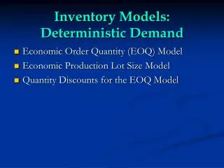
Cost Structures 4) Stockout costs are essentially the cost of losing current and or future business because items were not on hand when desired. Some of the costs mentioned here exhibit trade-offs. What I mean by this is that if we raise one type of cost we lower another type. As an example, as we increase the size of inventory and thus storage cost the stockout cost is lowered. With these ideas in mind we next study the economic order quantity model (EOQ). Note the assumptions of the model listed on page 338. In particular note demand has a constant rate and items are ordered in a fixed lot size.
EOQ In this model the total cost is made up of ordering cost plus carrying cost per year. The idea is to pick an order size, Q, that leads to the lowest total cost. Ordering costs per year = cost per order times orders per year. If D = the total demand in a year and Q is the amount ordered each time, then D/Q = the number of orders per year. With S the cost of placing an order, the ordering cost per year is S(D/Q). Carrying cost per year = annual carrying rate times unit cost times average inventory. Q/2 is the average inventory because at the beginning of the order period you have Q and at the end you have 0, (Q + 0)/2 = Q/2. We assume no quantity discounts so the unit cost will be called C and i is the carrying rate. Thus, the carrying cost = i(C)(Q/2).
EOQ Total cost = ordering cost + carrying cost = S(D/Q) + i(C)(Q/2) Now, we have said demand D is constant through the year. Thus the more that is ordered, Q, the less orders can be placed in the year. Thus, the higher the Q the lower the ordering cost. But, if Q is higher the carrying costs are higher. Thus we see a trade-off. When Q goes up order costs fall but carrying costs rise. Some really smart folks (Wilson and Harris) found the Q to order to give the lowest cost is Q = square root(2SD/iC).
EOQ Example Say a carpet store has demand for a certain type of carpet = 360 yards per year = D, it has a $10 cost per order = S, it as a 25% carrying cost = i, and the unit cost is $8 per yard = C. Thus the EOQ = Q = sqrt[{(2)(10)(360)}/{(.25)(8)}] = 60. Since the demand is 360 per year and it will order 60 units at a time it will order 360/60 = 6 times per year. Its total cost will be 10(360/60) + .25(8)(60/2) = 60 + 60 = 120. Just to show that this is the lowest TC, pick another Q (not using the EOQ formula) and see what is TC. I’ll try 40. TC = 10(360/40) + .25(8)(40/2) = 90 + 40 = 130. So, if you order less in an order you have to order more per year to meet the 360 level of demand. Order costs are higher but carrying costs shrink.
EOC example If you look at ordering 90 at a time you get TC = 10(360/90) + .25(8)(90/2) = 40 + 90. Thus, if a lot is ordered at one time you make fewer orders but you have a larger carrying cost. The EOQ formula shows us the Q that minimizes the total cost during the year.