Download
1 / 38
400 likes | 619 Vues
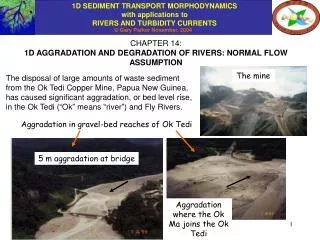
CHAPTER 14: 1D AGGRADATION AND DEGRADATION OF RIVERS: NORMAL FLOW ASSUMPTION. The mine. The disposal of large amounts of waste sediment from the Ok Tedi Copper Mine, Papua New Guinea, has caused significant aggradation, or bed level rise, in the Ok Tedi (“Ok” means “river”) and Fly Rivers.

E N D
CHAPTER 14: 1D AGGRADATION AND DEGRADATION OF RIVERS: NORMAL FLOW ASSUMPTION The mine The disposal of large amounts of waste sediment from the Ok Tedi Copper Mine, Papua New Guinea, has caused significant aggradation, or bed level rise, in the Ok Tedi (“Ok” means “river”) and Fly Rivers. Aggradation in gravel-bed reaches of Ok Tedi 5 m aggradation at bridge Aggradation where the Ok Ma joins the Ok Tedi
CHANNEL AGGRADATION AND FLOODPLAIN DEPOSITION OF OK TEDI AT GRAVEL-SAND TRANSITION Sediment depositing on the floodplain has destroyed the forest. River slope drops by an order of magnitude in the transition zone from braided gravel-bed to meandering sand-bed stream, leading to massive deposition of sand. Sand is dredged from the river to ameliorate the deposition.
RESPONSE OF A RIVER TO SUDDEN VERTICAL FAULTING CAUSED BY AN EARTHQUAKE View in November, 1999, shortly after the earthquake caused a sharp 3 m elevation drop at a fault. View in May, 2000 after aggradation and degradation have smoothed out the elevation drop. The above images of the Deresuyu River, Turkey, are courtesy of Patrick Lawrence and François Métivier (Lawrence, 2003)
RESPONSE OF A RIVER TO SUDDEN VERTICAL FAULTING CAUSED BY AN EARTHQUAKE contd. Inferred initial profile immediately after faulting in November, 1999 Profile in May, 2001 Upstream degradation (bed level lowering) and downstream aggradation (bed level increase) are realized as the river responds to the knickpoint created by the earthquake (Lawrence, 2003)
BACKGROUND AND ASSUMPTIONS • Change in channel bed level (aggradation or degradation) can occur in response to: • increase or decrease in upstream sediment supply; • change in hydrologic regime (water diversion or climate change); • change in river slope (e.g. channel straightening, as outlined in Chapter 2); • increased or decreased sediment supply from tributaries; • sudden inputs of sediment from debris flows or landslides; • faulting due to earthquakes or other tectonic effects such as tilting along the reach, • and; • changing base level at the downstream end of the reach of interest. Here “base level” loosely means a controlling elevation at the downstream end of the reach of interest. It means water surface elevation if the river flows into a lake or the ocean, or a downstream bed elevation controlled by e.g. tectonic uplift or subsidence at a point where the river is not flowing into standing water. Base level of this reach of the Eau Claire river, Wisconsin, USA is controlled by a reservoir, Lake Altoona
THE EQUILIBRIUM STATE contd. Rivers are different in many ways from laboratory flumes. It nevertheless helps to conceptualize rivers in terms of a long, straight, wide, rectangular flume with high sidewalls (no floodplain), constant width and a bed covered with alluvium. Such a “river” has a simple mobile-bed equilibrium (graded) state at which flow depth H, bed slope S, water discharge per unit width qw and bed material load per unit width qt remain constant in time t and in the streamwise direction x. A recirculating flume (with both water and sediment recirculated) at equilibrium is illustrated below.
THE EQUILIBRIUM STATE contd. The hydraulics of the equilibrium state are those of normal flow. Here the case of a plane bed (no bedforms) is considered as an example. The bed consists of uniform material with size D. The governing equations are (Chapter 5): Momentum conservation: Water conservation: Friction relations: where kc is a composite bed roughness which may include the effect of bedforms (if present). Generic transport relation of the form of Meyer-Peter and Müller for total bed material load: where t and nt are dimensionless constants:
THE EQUILIBRIUM STATE contd. In the case of the Chezy resistance relation, the equations governing the normal state reduce to: In the case of the Manning-Stickler resistance relation, the equations governing the normal state reduce with to: Let D, kc and R be given. In either case above, there are two equations for four parameters at equilibrium; water discharge per unit width qw, volume sediment discharge per unit width qt, bed slope S and flow depth H. If any two of the set (qw, qt, S and H) are specified, the other two can be computed. In a sediment-feed flume, qw and qt are set, and equilibrium S and H can be computed from either of the above pair. In a recirculating flume, qw and H are set (total water mass in flume is conserved), and qt and S can be computed.
THE EQUILIBRIUM STATE contd. The basic nature of the arguments of the previous slide do not change if a) total bed material transport is divided into bedload and suspended load components, each with its own predictor, b) bed shear stress is divided into skin friction and form drag, each with its own predictor, and c) transport/entrainment relations for uniform material are replaced with relations for sediment mixtures. Each new variable is accompanied by one new constraint (governing equation). For example, consider the case of gravel transport in the absence of bedforms. Using the gravel bedload transport relation of Powell et al. (2001) as an example, and setting kc = nkDs90 (no form drag), the problem reduces with the relations of Chapters 5 and 7 to Recalling that qbT = qbi and bedload fractions pi = qbi/qbT, if any two of the set (H, S, qw, qT) and either the bed surface fractions Fi or the bedload fractions pi are specified, the equilibrium values of the other parameters can be computed from the above equations. For example, if S, qw and Fi (from which Ds50 can be computed according to the relations of Chapter 2) are specified, H, qbT and pi can be computed directly from the above relations.
SIMPLIFICATIONS • The concepts of aggradation and degradation are best illustrated by using simplified relations for hydraulic resistance and sediment transport. Here the following simplifications are made in addition to the assumptions of constant width and the absence of a floodplain: • The case of a Manning-Strickler formulation with constant composite roughness kc is considered; • Bed material is taken to be uniform with size D; • The Exner equation of sediment conservation is based on a computation of total bed material load, which is computed via the generic equation • where s 1 is a constant to convert total boundary shear stress to that due to skin friction (if necessary). For example, to recover the corrected version of Meyer-Peter and Müller (1948) relation of Wong and Parker (submitted) for gravel transport, set t = 3.97 , nt = 1.5, c* = 0.0495 and s = 1. For the bed material load relation of Engelund and Hansen (1967) for sand transport, which uses total boundary shear stress, not that due to skin friction, • t = 0.05/Cf, nt = 2.5, c* = 0 and s = 1.
SIMPLIFICATIONS contd. 4. The full flood hydrograph or flow duration curve of discharge variation is replaced by a flood intermittency factor If, so that the river is assumed to be at low flow (and not transporting significant amounts of sediment) for time fraction 1 – If, and is in flood at constant discharge Q, and thus constant discharge per unit width qw = Q/B for time fraction If (Paola et al., 1992). The implied hydrograph takes the conceptual form below: In the long term, then, the relation between actual time t and time that the river has been in flood tf is given as Let the value of the total bed material load at flood flow qt be computed in m2/s. Then the total mean annual sediment load Gt in million tons per year is given as
SIMPLIFICATIONS contd. • There are many reasonable ways to compute the intermittency factor If. One reasonable way to do so is to: • compute the volume bed material transport rate Qtbf at bankfull flow; • use the full flow duration curve to compute the mean annual volume bed material transport rate Qtanav as • where qt,k denotes the value of qt in the kth discharge range, and pk denotes the fraction of time the flow is in this range, and • Compute the flood value of • qt and If as • In this way If denotes the fraction of time per year that continuous • bankfull flow would yield the annual sediment yield.
SIMPLIFICATIONS contd. It is important to realize that none of these simplifications are necessary. Once methods for computing aggradation and degradation are developed using the above simplifications, however, the analysis easily generalizes to cases with mixed grain sizes, a distinction between bedload and suspended bed material load, a computation of both form drag and skin friction, and computations using the full flow hydrograph or flow duration curve. The Minnesota River, USA near Le Sueur during the flood of record in 1965 Generalization to the case of varying width is also rather straightforward, and is implemented in future chapters of this e-book. Including the floodplain, however, is more difficult, especially in the case of meandering rivers. This is because when the floodplain is inundated and the floodplain depth is substantial, the thread of high velocity may no longer completely follow the river channel. The simplest reasonable assumption is that the bed material load at above-bankfull flows is equal to that at bankfull flow. channel
AGGRADATION AND DEGRADATION AS TRANSIENT RESPONSES TO IMPOSED DISEQIUILBRIUM CONDITIONS Aggradation or degradation of a river reach can be considered to be a response to disequilibrium conditions, by which the river tries to reach a new equilibrium. For example, if a river reach has attained an equilibrium with a given sediment supply from upstream, and that sediment supply is suddenly increased at t = 0, the river can be expected to aggrade toward a new equilibrium.
NORMAL FLOW FORMULATION OF MORPHODYNAMICS: GOVERNING EQUATIONS In this chapter the flow is calculated by approximating it with the normal flow formulation, even if the profile itself is in disequilibrium. The approximation is of loose validity in most cases of interest, and becomes more rigorously valid with increasing Froude number. Gradually varied flow is considered in Chapter 20. Using the Exner formulation of Chapter 2 and the Manning-Strickler formulation for flow resistance, the morphodynamic problem has the following character: In the above relations t denotes real time (as opposed to flood time) and the intermittency factor If accounts for the fact that the river is only occasionally in flood (and thus morphologically active).
THE NORMAL FLOW MORPHODYNAMIC FORMULATION AS A NONLINEAR DIFFUSION PROBLEM The previous formulation can be rewritten as: where d is a kinematic “diffusivity” of sediment (dimensions of L2/T) given by the relation The top equation is a diffusion equation. In the bottom equation, it is seen that d is dependent on S = - /x, so that the diffusion formulation is nonlinear. The problem is second-order in x and first order in t, so that one initial condition and two boundary conditions are required for solution.
INITIAL AND BOUNDARY CONDITIONS The reach over which morphodynamic evolution is to be described must have a finite length L. Here it extends from x = 0 to x = L. The initial condition is that of a specified bed profile; The simplest example of this is a profile with specified initial downstream elevation Id at x = L and constant initial slope SI; The upstream boundary condition can be specified in terms of given sediment supply, or feed rate qtf, which may vary in time; The simplest case is that of a constant value of sediment feed. The downstream boundary condition can be one of prescribed base level in terms of bed elevation; Again the simplest case is a constant value, e.g. d = 0.
NOTES ON THE DOWNSTREAM BOUNDARY CONDITION • In principle the best place to locate the downstream boundary condition is at a bedrock exposure, as illustrated below. In most alluvial streams, however, such points may not be available. Three alternatives are possible: • Set the boundary condition at a point so far downstream that no effect of e.g. changed sediment feed rate is felt during the time span of interest; • Set the boundary condition where the river joins a much larger river; or • Set the boundary condition at a point of known water surface elevation, such as a lake (see Chapter 20 and the use of the gradually varied flow model). Alluvial Kaiya River, Papua New Guinea, and downstream bedrock exposure Bedrock makes a good downstream b.c.
Feed sediment here! DISCRETIZATION FOR NUMERICAL SOLUTION The morphodynamic problem is nonlinear and requires a numerical solution. This may be done by dividing the domain from x = 0 to x = L into M subreaches bounded by M + 1 nodes. The step length x is then given as L/M. Sediment is fed in at an extra “ghost” node one step upstream of the first node. Bed slope can be computed by the relations to the right. Once the slope Si is computed the sediment transport rate qt,i can be computed at every node. At the ghost node, qt,g = qtf.
DISCRETIZATION OF THE EXNER EQUATION Let t denote the time step. Then the Exner equation discretizes to where and au is an upwinding coefficient. In a pure upwinding scheme, au = 1. In a central difference scheme, au = 0.5. A central difference scheme generally works well when the normal flow formulation is used. At the ghost node, qt,g = qtf. In computing qt,i/x at i = 1, the node at i – 1 (= 0) is the ghost node. At node M+1, the Exner equation is not implemented because bed elevation is specified as M+1 = d.
INTRODUCTION TORTe-bookAgDegNormal.xls The basic program in Visual Basic for Applications is contained in Module 1, and is run from worksheet “Calculator”. The program is designed to compute a) an ambient mobile-bed equilibrium, and b) the response of a reach to changed sediment input rate at the upstream end of the reach starting from t = 0. The first set of required input includes: flood discharge Q, intermittency If, channel (bankfull) width B, grain size D, bed porosity p, composite roughness height kc and ambient bed slope S (before increase in sediment supply). Composite roughness height kc should be equal to ks = nkD, where nk is in the range 2 – 4, in the absence of bedforms. When bedforms are expected kc should be estimated at bankfull flow using the techniques of Chapter 9 and 10 (compute Cz from hydraulic resistance formulation; kc = (11 H)/exp(Cz)). Various parameters of the ambient flow, including the ambient annual bed material transport rate Gt in tons per year, are then computed directly on worksheet “Calculator”.
INTRODUCTION TORTe-bookAgDegNormal.xls contd. The next required input is the annual average bed material feed rate Gtf imposed after t > 0. If this is the same as the ambient rate Gt then nothing should happen; if Gtf > Gt then the bed should aggrade, and if Gtf < Gt then it should degrade. The final set of input includes the reach length L, the number of intervals M into which the reach is divided (so that x = L/M), the time step t, the upwinding coefficient au (use 0.5 for a central difference scheme), and two parameters controlling output, the number of time steps to printout Ntoprint and the number of printouts (in addition to the initial ambient state) Nprint. The downstream bed elevation d is automatically set equal to zero in the program. Auxiliary parameters, including r (coefficient in Manning-Strickler), t and nt (coefficient and exponent in load relation), c* (critical Shields stress), s (fraction of boundary shear stress that is skin friction) and R (sediment submerged specific gravity) are specified in the worksheet “Auxiliary Parameters”.
INTRODUCTION TORTe-bookAgDegNormal.xls contd. The parameter s estimating the fraction of boundary shear stress that is skin friction, should either be set equal to 1 or estimated using the techniques of Chapter 9. In any given case it will be necessary to play with the parameters M (which sets x) and t in order to obtain good results. For any given x, it is appropriate to find the largest value of t that does not lead to numerical instability. The program is executed by clicking the button “Do a Calculation” from the worksheet “Calculator”. Output for bed elevation is given in terms of numbers in worksheet “ResultsofCalc” and in terms of plots in worksheet “PlottheData” The formulation is given in more detail in the worksheet “Formulation”, which is also available as a stand-alone document, Rte-bookAgDegNormalFormul.doc.
MODULE 1 Sub Main This is the master subroutine that controls the Visual Basic program. Sub Main() Clear_Old_Output Get_Auxiliary_Data Get_Data Compute_Ambient_and_Final_Equilibria Set_Initial_Bed_and_time Send_Output j = 0 For j = 1 To Nprint For w = 1 To Ntoprint Find_Slope_and_Load Find_New_eta Next w More_Output Next j End Sub
MODULE 1 Sub Set_Initial_Bed_and_time This subroutine sets the initial ambient bed profile. Sub Set_Initial_Bed_and_time() For i = 1 To N + 1 x(i) = dx * (i - 1) eta(i) = Sa * L - Sa * dx * (i - 1) Next i time = 0 End Sub
MODULE 1 Sub Find_Slope_and_Load This subroutine computes the load at every node. Sub Find_Slope_and_Load() Dim i As Integer Dim taux As Double: Dim qstarx As Double: Dim Hx As Double Sl(1) = (eta(1) - eta(2)) / dx Sl(M + 1) = (eta(M) - eta(M + 1)) / dx For i = 2 To M Sl(i) = (eta(i - 1) - eta(i + 1)) / (2 * dx) Next i For i = 1 To M + 1 Hx = ((Qf ^ 2) * (kc ^ (1 / 3)) / (alr ^ 2) / (B ^ 2) / g / Sl(i)) ^ (3 / 10) taux = Hx * Sl(i) / Rr / D If fis * taux <= tausc Then qstarx = 0 Else qstarx = alt * (fis * taux - tausc) ^ nt End If qt(i) = ((Rr * g * D) ^ 0.5) * D * qstarx Next i End Sub
MODULE 1 Sub Find_New_eta This subroutine implements the Exner equation to find the bed one time step later. Sub Find_New_eta() Dim i As Integer Dim qtback As Double: Dim qtit As Double: Dim qtfrnt As Double: Dim qtdif As Double For i = 1 To M If i = 1 Then qtback = qqtf Else qtback = qt(i - 1) End If qtit = qt(i) qtfrnt = qt(i + 1) qtdif = au * (qtback - qtit) + (1 - au) * (qtit - qtfrnt) eta(i) = eta(i) + dt / (1 - lamp) / dx * qtdif * Inter Next i time = time + dt End Sub
A SAMPLE COMPUTATION The ambient sediment transport rate is 305,000 tons/year. At time t = 0 this is increased to 700,000 tons per year. The bed must aggrade in response.
INTERPRETATION The long profile of a river is a plot of bed elevation versus down-channel distance x. The long profile of a river is called upward concaveif slope S = -/x is decreasing in the streamwise direction; otherwise it is called upward convex. That is, a long profile is upward concave if Aggrading reaches often show transient upward concave profiles. This is because the deposition of sediment causes the sediment load to decrease in the downstream direction. The decreased load can be carried with a decreased Shields number *, and thus according to the normal-flow formulation of the present chapter, a decreased slope:
INTERPRETATION contd. The transient long profile of Slide 29 is upward concave because the river is aggrading toward a new mobile-bed equilibrium with a higher slope. Once the new equilibrium is reached, the river will have a constant slope (vanishing concavity). This process is outlined in the next slide (Slide 32), in which all the input parameters are the same as in Slide 28 except Ntoprint, which is varied so that the duration of calculation ranges from 1 year (far from final equilibrium) to 250 years (final equilibrium essentially reached). Slide 33 shows a case where the profile degrades to a new mobile-bed equilibrium. During the transient process of degradation the long profile of the bed is downward concave, or upward convex. This is because the erosion which drives degradation causes the load, and thus the slope to increase in the downstream direction. The input conditions for Slide 32 are the same as that of Slide 28, except that the sediment feed rate Gtf is dropped to 70,000 tons per year. This value is well below the ambient value of 305,000 tons per year (see Slide 28), forcing degradation and transient downward concavity. In addition, Ntoprint is varied so that the duration of calculation varies from 1 year to 250 years. It will be seen in Chapter 25 that factors such as subsidence or sea level rise can drive equilibrium long profiles which are upward concave.
ADJUSTING THE NUMBER M OF SPATIAL INTERVALS AND THE TIME STEP t The calculation becomes unstable, and the program crashes if the time step t is too long. The above example resulted in a crash when t was increased from the value of 0.01 years in Slide 29 to 0.05 years. The larger the value M of spatial intervals is, the smaller is the maximum value of t to avoid numerical instability. Acceptable values of M and t can be found by trial and error.
AN EXTENSION: RESPONSE OF AN ALLUVIAL RIVER TO VERTICAL FAULTING DUE TO AN EARTHQUAKE The code in RTe-bookAgDegNormal.xls represents a plain vanilla version of a formulation that is easily extended to a variety of other cases. The spreadsheet RTe-bookAgDegNormalFault.xls contains an extension of the formulation for sudden vertical faulting of the bed. The bed downstream of the point x = rfL (0 < rf < 1) is suddenly faulted downward by an amount f at time tf. The eventual smearing out of the long profile is then computed.
RESULTS OF SAMPLE CALCULATION WITH FAULTING contd. In time the fault is erased by degradation upstream and aggradation downstream, and a new mobile-bed equilibrium is reached.
REFERENCES FOR CHAPTER 14 Engelund, F. and E. Hansen, 1967, A Monograph on Sediment Transport in Alluvial Streams, Technisk Vorlag, Copenhagen, Denmark. Lawrence, P., 2003, Bank Erosion and Sediment Transport in a Microscale Straight River, Ph.D. thesis, University of Paris 7 – Denis Diderot, 167 p. Meyer-Peter, E. and Müller, R., 1948, Formulas for Bed-Load Transport, Proceedings, 2nd Congress, International Association of Hydraulic Research, Stockholm: 39-64. Paola, C., Heller, P. L. & Angevine, C. L., 1992, The large-scale dynamics of grain-size variation in alluvial basins. I: Theory, Basin Research, 4, 73-90. Powell, D. M., Reid, I. and Laronne, J. B., 2001, Evolution of bedload grain-size distribution with increasing flow strength and the effect of flow duration on the caliber of bedload sediment yield in ephemeral gravel-bed rivers, Water Resources Research, 37(5), 1463-1474. Wong, M. and Parker, G., submitted, The bedload transport relation of Meyer-Peter and Müller overpredicts by a factor of two, Journal of Hydraulic Engineering, downloadable at http://cee.uiuc.edu/people/parkerg/preprints.htm .