Enhancing Alloy Design with FactOptimal: Optimal Conditions and Thermodynamic Insights
The FactOptimal module optimizes alloy and process design by utilizing thermodynamic and property databases, coupled with FactSage software and the Mesh Adaptive Direct Search Algorithm. This module assists in identifying the best conditions for alloys through a systematic approach, providing numerous examples such as maximizing flame temperatures and calculating minimum liquidus temperatures under constraints. Improved capabilities in the latest version, FactOptimal 6.4, include double-target calculations, additional optimizable properties, and enhanced reporting of results for better usability.

Enhancing Alloy Design with FactOptimal: Optimal Conditions and Thermodynamic Insights
E N D
Presentation Transcript
The FactOptimal Module FactOptimal is programmed to identify the optimal conditions for alloy and process design using thermodynamic and property databases, FactSage software and the Mesh Adaptive Direct Search Algorithm. A.Gheribi, E. Bélisle, C.W. Bale and A.D. Pelton CRCT, Ecole Polytechnique de Montréal S. Le Digabel and C. Audet, GERAD, Ecole Polytechnique de Montréal Table of contents Section 1 Introduction Section 2How does FactOptimal Work – Using the stored examples Section 3 Example 1 : Maximize an adiabatic flame temperature Section 4Example 2 : Calculation of minimum liquidus temperature under constraints Section 5 Example 3 : How to use equality constraints Section 6 Example 4 : FactOptimal coupled with solidification software Section 7 Introduction to the Pareto concept Section 8Example 5 : Optimize 2 properties with two files (linked) Pgas vs density (T2 = T1+20) Section 9Example 6 : Application using the cache option (Next Run) Section 10Example 7 :Target optimization Section 11Optimization using the Function Builder Section 12Example 8 : Calculation of characteristic points on the liquidus surface Section 13Characteristic points – reciprocal systems
The FactOptimal Module Table of contents (cont.) Section 14 Example 9 : Characteristic points – closest characteristic point Section 15Example 10: Improve the mechanical properties of AZ91 by addition of Ca and RE Section 16 Example 11 : Improvement of the mechanical properties of 7178 aluminum alloy Section 17Example 12 : Improve the texture and grain refinement properties at low temperature Section 18 Example 13 : Minimize the liquidus temperature and minimize the solid fraction 200 oC below the liquidus Section 19 Example 14: Double target optimization
Introduction - 1 - The Equilib module can be used to screen potential systems, searching for compositions having a desired set of properties and phase constitution, under a given set of constraints • For instance, one could search for alloys within a given composition range, with a liquidus temperature below xoC, with a desired freezing range, with a maximum or minimum amount of precipates after annealing at yoC, with a density or shrinkage ratio within a given range, etc. One could also search for optimal annealing or rolling temperatures, for example. • However, to perform such searches “by hand” for a multicomponent alloy by simply performing thousands of calculations over a grid of compositions is extremely time-consuming. • - FactOptimalextends the capability of Equilib by coupling it with a Mesh Adaptive Direct Search method algorithm (MADS) developed at GERAD by S. Le Digabel and C. Audet, Ecole Polytechnique de Montreal 1.1 FactOptimal
The FactOptimal Module What’s New In FactOptimal 6.4 ? • Double Target calculations: one can now target twoproperties simultaneously. • Continue run after a target calculation: it is now possible to click on “continue run” to calculate another composition corresponding to the desired target. • Additional properties for optimization or constraints : physical properties (density, thermal expansion, viscosity, thermal conductivity, electrical conductivity…) are now available. • For cooling calculations, the annealing temperature can now be chosen as an optimizable variable. • Logarithmic values: one can optimize the logarithm of a property e.g log(activity) or log(P). In certain cases this may present a numerical advantage, increasing speed and precision. • When using two input files, the "linked" button previously allowed using the temperature from the first file as a variable for the second file. In FactOptimal 6.4, amount of reactants and pressure can also be used. • A function saved with Function Builder can now be used as a property constraint. • When characteristic points on a liquidus surface are calculated, the results are now shown in a table as well as on a graph, displaying detailed compositions, temperature and the solid phases in equilibrium with the liquid. 1.2 FactOptimal
The FactOptimal Module What’s New In FactOptimal 6.4 ? (cont.) • There is now an option to calculate the minimum or maximum on a liquidus surface closest to the initial composition. • When calculating characteristic points on a liquidus surface, there is a new option either to calculate the lowest minimum first or to calculate all minima with no priority. • There is a new parameter to limit the maximum time for the optimization. • When working with variables of type “real”, a new parameter is available: the decimal precision. • Results displayed in a table (target type calculations or characteristic points on a liquidus. surface) can now be saved as an Excel file. • When using two input files, property constraints can now be applied on either file. • When no feasible solution is found, FactOptimal now displays the closest solution (example on page 4.20). 1.3 FactOptimal
The FactOptimal Module What was New In FactOptimal 6.3 ? • Target calculations : in addition to minimizing/maximizing one can now target a specific value. • Additional new property for optimization : activity of a phase/species. • Additional new variables : temperature and pressure. • Additional new property constraint : activity of a phase/species. • The sum of composition variables can now be greater than 1. • Thus, variables can now be of type integer or real. • When using two input files, the "linked" button is now activated in order to use the temperature from the first file in the second file. • When using two input files, properties constraints can now apply to each of the input files. • Latest optimizations are saved with Equilib files and can be recalled by using the “Recent” button • Convenient MIN/MAX buttons to set all minimum/maximum values of composition variables • For a Scheil cooling system, the mass of specific species/phase(s) can now be optimized • Better optimization for composition constraints having equality rules • Table display of result for the special points option • Use of cache file to restart any optimization from the latest calculation 1.4 FactOptimal
General recommendations • In general, we recommend that you perform every optimization twice, using different starting points. • If you are not sure of the best starting point, a good practice is to use the Q-Random option. See p. 3.8 and p. 19.5 for detailed examples. • Do not hesitate to use the « Continue Run >> » option to make sure there is no better answer when you have completed the maximum number of calculations entered in the parameters (see example 6). • If you need more information or if you have specific questions about FactOptimal, please contact Aimen Gheribi (aimen.gheribi@polymtl.ca) or Eve Bélisle (eve.belisle@polymtl.ca). 1.5 FactOptimal
Introduction - 2 • The purpose of FactOptimal is to minimize and/or maximize a set of functions: {f1(x1,x2..T, P); f2(x1,x2….T, P)} • The functions are calculated by Equilib • The functions may be non-smooth (e.g. liquidus ) • The estimation of derivatives is problematic • Evaluations of f can be time consuming • The function calculation may fail unexpectedly at some points • The constraints may be non-linear, non-smooth or Boolean 1.6 FactOptimal
How does FactOptimalwork ? – 1 . NOMAD(Nonsmooth Optimization by Mesh Adaptive Direct Search) Commands FactOptimal Text file In memory XML macro processing Equilib Calculator (bb.dll) XML FactOptimal 2.1
How does FactOptimalwork ? – 2 The principal of the optimization is a loop where FactOptimal sends compositions to Equilib, then Equilib returns the values of the properties to be optimized to FactOptimal. This is repeated until the properties minimum or maximum of is reached. For example, the minimization of the liquidus temperature of the KCl-RbCl-CsCl salt system can be represented by : FactOptimal 2.2
Using the stored examples The following examples are stored on your computer. In Equilib click on ‘File > Open > Directory > Fact Optimal Examples’ > Fact Optimal 1 (Maximum adiabatic ...’). In the Menu Window click on ‘Calculate ’ and then in the Results Window click the FactOptimal icon. In the Fact Optimal Window click on ‘Recent ...’to load the stored example. FactOptimal 2.3
Example 1: Maximize an adiabatic flame temperature - 1 The objective is to maximize the adiabatic flame temperature of :(1-A) CH4 + (A) O2 By varying A from 0 to 1 in steps of 0.01, you can calculate the adiabatic flame temperature as a function of Ausing the Equilib module (see Equilib regular slide show, section 10). Plotting the results you find that: Tad ,max ~3075 K when A ~0.65 FactOptimal 3.1
Example 1: Maximize an adiabatic flame temperature - 2 To calculate the maximum temperature with FactOptimal, the first stepis to perform a single equilibrium calculation at any arbitrary composition and then open FactOptimal. FactOptimal Icon FactOptimal 3.2
Example 1: Maximize an adiabatic flame temperature - 3 When you “click” on the FactOptimalicon the first window of the module appears. If you are using the stored example files, click on “Recent...” to load the FactOptimal file. There are 5 tabs. The first tab is “Properties” where we define the quantities to minimize and/or maximize. In this example, we specify that : 1 - we consider one property 2 - we want to maximize this property 3 - the property is temperature 1 2 3 Click on Next to go to the Variables tab FactOptimal 3.3
Example 1: Maximize an adiabatic flame temperature - 4 In the “Variables” tab we define the permissible range of composition and the initial values for the first estimate. Alternatively, select “Q-Random” and let the program choose the initial values. (see page 3.8) Use “ALL” buttons to set the same value for all variables. REAL type is chosen with values varying from 0 to 1. For INTEGER type, see example in section 3.7. Only composition variables are used in this example. Click on Next to go to the Constraints tab. FactOptimal 3.4
Example 1: Maximize an adiabatic flame temperature - 5 In the “Constraints” tab the sum of composition variables is set by default to 1. In the “Parameters” tab we define the maximum number of Equilib calculations and the search region. If the initial point is a good estimate of the expected answer, choose Small (0.1), otherwise choose Large (1) or Medium (0.5). The program will stop after the selected maximum number of Equilib calculations, or it may converge earlier. The number of calculations can be extended later if desired without losing the first set of calculations. Similarly, the stop button can be used at any time to terminate the optimization calculations. See section 9 for more details. Click on the “Calculate >>” button to start the optimization. FactOptimal 3.5
Example 1: Maximize an adiabatic flame temperature - 6 We obtain the results after 25 Equilib Calculations. The Equilib Results Window with the equilibrium calculation corresponds to the calculated maximum adiabatic flame temperature. FactOptimal 3.6
Example 1: Maximize an adiabatic flame temperature - 7 To decrease the number of significant digits and thereby decrease the computation time, you can choose to work with INTEGER type variables. Using the same example, INTEGER type is chosen with values varying from 0 to 1000. By selecting this option as opposed to real values varying from 0 to 1, we are limiting the number of significant digits to 3. FactOptimal 3.7
Example 1: Maximize an adiabatic flame temperature - 8 We also clicked the Q-Random (Quasi-Random) option, in order to let FactOptimal determine the best initial point. This is a good practice if you are not sure of what the best starting point should be. When choosing this option, we have to define the number of such calculations. In the present example 50 quasi-random calculations will be performed in order to get the best initial point, then 25 subsequent Equilib calculations will be performed to determine the best solution for a total of 75 calculations. FactOptimal 3.8
In this section we will calculate the minimum liquidus temperature of a multicomponent solution phase under various constraints of composition, cost, density, etc. There are 2 examples – Example 2: Minimize the liquidus temperature under constraints • minimize the liquidus temperature of an Al-Cu-Mg-Zn molten alloy using data from FTlite • minimize the liquidus temperature of a LiCl-NaCl-KCl-LiF-NaF-KF molten salt using data from FTsalt
Example 2a : Minimize the alloy liquidus temperature under constraints - 1 System: Al-Cu-Mg-Zn. Constraints: Step 1:Using Equilib define the system and select the appropriate database: FTlite. • Sum of mole fractions (XAl + XCu) < 0.2 • Density < 2.2 g/ml • Cost < 2900 $/ton FactOptimal 4.1
Example 2a : Minimize the alloy liquidus temperature under constraints - 2 Step 2: Perform a single equilibrium calculation at an arbitrary composition and specify a precipitate (P) calculation on the liquid (i.e. liquidus temperature calculation) and “include molar volumes” (for the calculation of the density): FactOptimal 4.2
Example 2a : Minimize the alloy liquidus temperature under constraints - 3 Equilib Results Window Click on the FactOptimal icon FactOptimal 4.3
Example 2a : Minimize the alloy liquidus temperature under constraints - 4 Step 3: Click on the FactOptimal icon and set up the calculation. If you are using the stored example files, click on “Recent...” to load the Fact Optimal file. In this example, we specify that: • we consider one property • we want to minimize this property • the property is Temperature • the Costis to be included in the optimization 1 2 3 4 FactOptimal 4.4
Example 2a : Minimize the alloy liquidus temperature under constraints - 5 Step 4: In the "Variables" tab we define the permissible composition range (and initial estimates) 0.05 ≤ Wt.% Al ≤ 0.2 (0.05)0.05 ≤ Wt.% Cu ≤ 0.2 (0.02)0.75 ≤ Wt.% Mg ≤ 0.9 (0.75)0.00 ≤ Wt.% Zn ≤ 0.15 (0.03) FactOptimal 4.5
Example 2a : Minimize the alloy liquidus temperature under constraints - 6 Step 5: In the "cost" tab we define the unit price of each component. The cost per unit can be in $/ton, $/kg or $/g $2132 per ton Al$7315 per ton Cu$2980 per ton Mg$2100 per ton Zn FactOptimal 4.6
Example 2a : Minimize the alloy liquidus temperature under constraints - 7 Step 6: Define the constraints on composition: X(Al) + X(Cu) < 0.2 SUM (Comp. Variables) = 1 therefore compositions are mole fractions FactOptimal 4.7
Example 2a : Minimize the alloy liquidus temperature under constraints - 8 Step 7: Define the constraints on properties :r < 2.2 g/ml cost < 2900 $/Ton FactOptimal 4.8
Example 2a : Minimize the alloy liquidus temperature under constraints - 9 Step 8: Enter the maximum number of Equilib calculations and the initial search region (see slide 3.5). The max number of calculations is 150 because previous calculations have shown this number is necessary to obtain convergence. FactOptimal 4.9
Example 2a : Minimize the alloy liquidus temperature under constraints - 10 FactOptimal Results Window Save and print the graph or change the axis scale Minimum Composition at the minimum Values of the defined constraints: X(Al) + X(Cu) < 0.2 r < 2.2 g/ml cost < 2900 $/Ton FactOptimal 4.10
Example 2a : Minimize the alloy liquidus temperature under constraints - 11 Equilib Results Window FactOptimal 4.11
Example 2b: Minimize the salt liquidus temperature under constraints - 1 This is a typical problem to solve for the design of a molten salt medium for thermal storage System: LiCl-NaCl-KCl-LiF-NaF-KF Constraints: Step 1:Using Equilib, define the system and select the appropriate database: FTsalt. • wt.%(LiCl) + wt.%(LiF) ≤ 10 • wt.%(NaCl) + wt.%(KCl) ≥ 3*(wt.%(NaF) + wt.%(KF)) • Density ≥ 1750 kg/m3 • Cp ≥ 1250 J/kg • Cost ≤ 3.5 $/kg Use a basis of 1000g FactOptimal 4.12
Example 2b: Minimize the salt liquidus temperature under constraints - 2 Step 2: Perform a single equilibrium calculation at an arbitrary composition and specify a precipitate (P) calculation on the liquid (i.e. liquidus temperature calculation) and “include molar volumes” (for the calculation of the density): FactOptimal 4.13
Example 2b: Minimize the salt liquidus temperature under constraints - 4 Step 3: After doing one calculation, click on the FactOptimal icon and set up the optimization. If you are using the stored example files, click on “Recent...” to load the Fact Optimal file. In this example, we specify that: • we consider one property • we want to minimize this property • the property is Temperature • the Costis to be included in the optimization 1 2 3 4 FactOptimal 4.14
Example 2b: Minimize the salt liquidus temperature under constraints - 5 Step 4: Define the permissible composition range and a set of initial estimates. Here we are not sure of the best starting point so we used the Q-Random option. FactOptimal 4.15
Example 2b: Minimize the salt liquidus temperature under constraints - 6 Step 5:In the "cost" tab we define the unit price of each component. FactOptimal 4.16
Example 2b: Minimize the salt liquidus temperature under constraints - 7 Step 5: Define the constraints on composition. • Sum (Comp. Variables) = 1000 g • wt.%(LiCl) + wt.%(LiF) ≤ 10 • wt.%(NaCl) + wt.%(KCl) ≥ 3*(wt.%(NaF) + wt.%(KF)) FactOptimal 4.17
Example 2b: Minimize the salt liquidus temperature under constraints - 8 Step 6: Define the constraints on properties. • Density ≥ 1750 kg/m3 • Cp ≥ 1250 J/kg • Cost ≤ 3.5 $/kg FactOptimal 4.18
Example 2b: Minimize the salt liquidus temperature under constraints - 9 Step 7: Enter the maximum number of Equilib calculations and the initial search region (see slide 3.5). Here we tried 500 calculations with 500 Quasoi-Random calcuations for a total of 1000 calculations. We used a large search region. FactOptimal 4.19
Example 2b: Minimize the salt liquidus temperature under constraints - 10 FactOptimal Results Window: Unfortunately, after 1000 calculations, FactOptimal did not find any answer respecting the constraints. Here the closest results are shown in a table. FactOptimal 4.20
Example 2b: Minimize the salt liquidus temperature under constraints - 11 Here we change constraints on composition and cost. • The new constraints are : • wt.%(LiCl) + wt.%(LiF) ≤ 100 • wt.%(NaCl) + wt.%(KCl) ≥ (NaF + KF) • Density ≥ 1750 kg/m3 • Cp ≥ 1250 J/kg • Cost ≤ 5.5 $/kg FactOptimal 4.21
Example 2b: Minimize the salt liquidus temperature under constraints - 12 FactOptimal Results Window:with the new set of constraints, FactOptimal finds the lowest liquidus temperature to be577.39ºC. FactOptimal 4.22
Example 2b: Minimize the salt liquidus temperature under constraints - 13 Equilib Results Window FactOptimal 4.23
Example 3 : How to use equality constraints - 1 Using the example from section 3, we will calculate the maximum adiabatic flame temperature when O2 is replaced by air where moles O2 = moles N2/4. FactOptimal 5.1
Example 3 : How to use equality constraints - 2 We want the following constraints to be respected (molar basis): CH4 + O2 + N2 = 1 O2 = N2/4 To enter these constraints in FactOptimal, they must be converted to allow only one degree of freedom : O2 = -1/5*CH4 + 1/5 N2 = -4/5*CH4 + 4/5 That is, if there are m composition variables (C1, C2, ... Cm) and n equations relating these variables, then the first (m-n) variables must be expressed as functions of the remaining variables as Ci = f(Cm-n+1,...Cm); i ≤ (m-n) FactOptimal 5.2
Example 3 : How to use equality constraints - 3 The SUM (Comp. variables) option must always be unchecked when equality constraints are being used. FactOptimal 5.3
Example 3 : How to use equality constraints - 4 The adiabatic flame temperature in air is less than in O2. FactOptimal 5.4
Example 4 : Maximize the total mass of all precipitates in the hcp matrix for an (AZ31+Ce) Mg-based alloy after Scheil-Gulliver cooling and subsequent full annealing - 1 System: Al-Ce-Mg-Zn Step 1: Using Equilib we define the system and select the appropriate databases FTlite. The arbitrary composition corresponds to approximately the composition of AZ31 alloys. FactOptimal 6.1
Example 4 : Maximize the total mass of all precipitates in the hcp matrix for an (AZ31+Ce) Mg-based alloy after Scheil-Gulliver cooling and subsequent full annealing - 2 Step 2: Perform a single Equilib calculation using the solidification software and choosing a Scheil-Gulliver Cooling type calculation (see Equilib Advanced Slide Show, slide 13.1) FactOptimal 6.2


![Wrangling the [Biblio] Module](https://cdn1.slideserve.com/2444107/wrangling-the-biblio-module-dt.jpg)