Download

1 / 44
440 likes | 577 Vues
7-1 Aggregate Supply. The aggregate supply relation captures the effects of output on the price level. It is derived from the behavior of wages and prices. Recall the equations for wage and price determination from Chapter 6:. 7-1 Aggregate Supply.

E N D
7-1 Aggregate Supply • The aggregate supply relation captures the effects of output on the price level. It is derived from the behavior of wages and prices. • Recall the equations for wage and price determination from Chapter 6:
7-1 Aggregate Supply • Step 1: Eliminate the nominal wage from: and then In words, the price level depends on the expected price level and the unemployment rate. We assume that and z are constant.
7-1 Aggregate Supply • Step 2: Express the unemployment rate in terms of output: Therefore, for a given labor force, the higher is output, the lower is the unemployment rate.
7-1 Aggregate Supply • Step 3: Replace the unemployment rate in the equation obtained in step one gives us the aggregate supply relation: In words, the price level depends on the expected price level, Pe, and the level of output, Y (and also , z, and L, but we take those as constant here).
7-1 Aggregate Supply • The AS relation has two important properties: • An increase in output leads to an increase in the price level. This is the result of four steps: • An increase in output leads to an increase in employment. • The increase in employment leads to a decrease in unemployment and therefore to a decrease in the unemployment rate. • The lower unemployment rate leads to an increase in the nominal wage. • The increase in the nominal wage leads to an increase in the prices set by firms and therefore to an increase in the price level.
7-1 Aggregate Supply • The second property of the AS relation is that: • An increase in the expected price level leads, one for one, to an increase in the actual price level. This effect works through wages: • If wage setters expect the price level to be higher, they set a higher nominal wage. • The increase in the nominal wage leads to an increase in costs, which leads to an increase in the prices set by firms and a higher price level.
7-1 Aggregate Supply Figure 7 - 1 The Aggregate Supply Curve Given the expected price level, an increase in output leads to an increase in the price level. If output is equal to the natural level of output, the price level is equal to the expected price level.
7-1 Aggregate Supply • The AS curve has three properties that will prove useful in what follows: • The aggregate supply curve is upward sloping. Put another way, an increase in output, Y, leads to an increase in the price level, P. • The aggregate supply curve goes through point A, where Y = Ynand P = Pe. • An increase in the expected price level, Pe, shifts the aggregate supply curve up. Conversely, a decrease in the expected price level shifts the aggregate supply curve down.
7-1 Aggregate Supply Figure 7 - 2 The Effect of an Increase in the Expected Price Level on the Aggregate Supply Curve An increase in the expected price level shifts the aggregate supply curve up.
7-1 Aggregate Supply • Let’s summarize: • Starting from wage determination and price determination in the labor market, we have derived the aggregate supply relation. • This means that for a given expected price level, the price level is an increasing function of the level of output. It is represented by an upward-sloping curve, called the aggregate supply curve. • Increases in the expected price level shift the aggregate supply curve up; decreases in the expected price level shift the aggregate supply curve down.
7-2 Aggregate Demand • The aggregate demand relation captures the effect of the price level on output. It is derived from the equilibrium conditions in the goods and financial markets described in Chapter 5:
7-2 Aggregate Demand Figure 7 - 3 The Derivation of the Aggregate Demand Curve An increase in the price level leads to a decrease in output.
7-2 Aggregate Demand • Changes in monetary or fiscal policy—or more generally in any variable, other than the price level, that shift the IS or the LM curves—shift the aggregate demand curve. • The IS curve is downward sloping, the LM curve is upward sloping. • The negative relation between output and the price level is drawn as the downward-sloping curve AD.
7-2 Aggregate Demand Figure 7 - 4 Shifts of the Aggregate Demand Curve At a given price level, an increase in government spending increases output, shifting the aggregate demand curve to the right. At a given price level, a decrease in nominal money decreases output, shifting the aggregate demand curve to the left.
7-2 Aggregate Demand • Let’s summarize: • Starting from the equilibrium conditions for the goods and financial markets, we have derived the aggregate demand relation. • This relation implies that the level of output is a decreasing function of the price level. It is represented by a downward-sloping curve, called the aggregate demand curve. • Changes in monetary or fiscal policy – or more generally in any variable, other than the price level, that shifts the IS or the LM curves – shift the aggregate demand curve.
7-3 Equilibrium in the Short Runand in the Medium Run • Equilibrium depends on the value of Pe. The value of Pe determines the position of the aggregate supply curve, and the position of the AS curve affects the equilibrium.
7-3 Equilibrium in the Short Runand in the Medium Run Figure 7 - 5 The Short-Run Equilibrium Equilibrium in the Short Run The equilibrium is given by the intersection of the aggregate supply curve and the aggregate demand curve. At point A, the labor market, the goods market, and financial market are all in equilibrium. • The aggregate supply curve AS is drawn for a given value of Pe. The higher the level of output, the higher the price level. • The aggregate demand curve AD is drawn for given values of M, G, and T. The higher the price level is, the lower the level of output.
7-3 Equilibrium in the Short Runand in the Medium Run From the Short Run to the Medium Run At point A, Wage setters will revise upward their expectations of the future price level. This will cause the AS curve to shift upward. Expectation of a higher price level also leads to a higher nominal wage, which in turn leads to a higher price level.
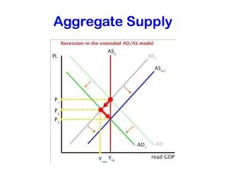
7-3 Equilibrium in the Short Runand in the Medium Run Figure 7 - 6 The Adjustment of Output over Time From the Short Run to the Medium Run If output is above the natural level of output, the AS curve shifts up over time until output has fallen back to the natural level of output. The adjustment ends once wage setters no longer have a reason to change their expectations. In the medium run, output returns to the natural level of output.
7-3 Equilibrium in the Short Runand in the Medium Run From the Short Run to the Medium Run • Let’s summarize: • In the short run, output can be above or below the natural level of output. Changes in any of the variables that enter either the aggregate supply relation or the aggregate demand relation lead to changes in output and to changes in the price level. • In the medium run, output eventually returns to the natural level of output. The adjustment works through changes in the price level.
7-4 The Effects of a Monetary Expansion The Dynamics of Adjustment • In the aggregate demand equation, we can see that an increase in nominal money, M, leads to an increase in the real money stock, M/P, leading to an increase in output. The aggregate demand curve shifts to the right.
7-4 The Effects of a Monetary Expansion The Dynamics of Adjustment The increase in the nominal money stock causes the aggregate demand curve to shift to the right. In the short run, output and the price level increase.
7-4 The Effects of a Monetary Expansion Figure 7 - 7 The Dynamic Effects of a Monetary Expansion The Dynamics of Adjustment A monetary expansion leads to an increase in output in the short run but has no effect on output in the medium run. The difference between Y and Yn sets in motion the adjustment of price expectations. In the medium run, the AS curve shifts to AS’’ and the economy returns to equilibrium at Yn. The increase in prices is proportional to the increase in the nominal money stock.
7-4 The Effects of a Monetary Expansion Going Behind the Scenes • The impact of a monetary expansion on the interest rate can be illustrated by the IS-LM model. • The short-run effect of the monetary expansion is to shift the LM curve down. The interest rate is lower, output is higher. • If the price level did not increase, the shift in the LM curve would be larger—to LM’’.
7-4 The Effects of a Monetary Expansion Figure 7 - 8 The Dynamic Effects of a Monetary Expansion on Output and the Interest Rate Going Behind the Scenes The increase in nominal money initially shifts the LM curve down, decreasing the interest rate and increasing output. Over time, the price level increases, shifting the LM curve back up until output is back at the natural level of output.
7-4 The Effects of a Monetary Expansion The Neutrality of Money • In the short run, a monetary expansion leads to an increase in output, a decrease in the interest rate, and an increase in the price level. • In the medium run, the increase in nominal money is reflected entirely in a proportional increase in the price level. The increase in nominal money has no effect on output or on the interest rate. • The neutrality of money in the medium run does not mean that monetary policy cannot or should not be used to affect output.
7-5 A Decrease in the Budget Deficit Figure 7 - 9 The Dynamic Effects of a Decrease in the Budget Deficit A decrease in the budget deficit leads initially to a decrease in output. Over time, however, output returns to the natural level of output.
How Long Lasting Are the Real Effects of Money? Figure 1 The Effects of an Expansion in Nominal Money in the Taylor Model Macroeconometric models are larger-scale versions of the aggregate supply and aggregate demand model in this chapter. They are used to answer questions such as how long the real effects of money last.
7-5 A Decrease in the Budget Deficit Deficit Reduction, Output, and the Interest Rate Since the price level declines in response to the decrease in output, the real money stock increases. This causes a shift of the LM curve to LM’. Both output and the interest rate are lower than before the fiscal contraction.
7-5 A Decrease in the Budget Deficit Figure 7 - 10 The Dynamic Effects of a Decrease in the Budget Deficit on Output and the Interest Rate Deficit Reduction, Output, and the Interest Rate A deficit reduction leads in the short run to a decrease in output and to a decrease in the interest rate. In the medium run, output returns to its natural level, while the interest rate declines further.
7-5 A Decrease in the Budget Deficit Deficit Reduction, Output, and the Interest Rate • The composition of output is different than it was before deficit reduction. • Income and taxes remain unchanged, thus, consumption is the same as before. • Government spending is lower than before; therefore, investment must be higher than before deficit reduction—higher by an amount exactly equal to the decrease in G.
7-5 A Decrease in the Budget Deficit Budget Deficits, Output, and Investment Let’s summarize: • In the short run, a budget deficit reduction, if implemented alone leads to a decrease in output and may lead to a decrease in investment. • In the medium run, output returns to the natural level of output, and the interest rate is lower. A deficit reduction leads unambiguously to an increase in investment. • It is easy to see how our conclusions would be modified if we did take into account the effects on capital accumulation. In the long run, the level of output depends on the capital stock in the economy.
7-6 Changes in the Price of Oil Figure 7 - 11 The Real Price of Oil Since 1970 There were two sharp increases in the relative price of oil in the 1970s, followed by a decrease until the 1990s, and a large increase since then. Each of the two large price increases of the 1970s was associated with a sharp recession and a large increase in inflation—a combination macroeconomists call stagflation, to capture the combination of stagnation and inflation that characterized these episodes.
7-6 Changes in the Price of Oil Figure 7 - 12 The Effects of an Increase in the Price of Oil on the Natural Rate of Unemployment Effects on the Natural Rate of Unemployment An increase in the price of oil leads to a lower real wage and a higher natural rate of unemployment.
7-6 Changes in the Price of Oil The Dynamics of Adjustment • An increase in the markup, , caused by an increase in the price of oil, results in an increase in the price level, at any level of output, Y. The aggregate supply curve shifts up.
7-6 Changes in the Price of Oil The Dynamics of Adjustment After the increase in the price of oil, the new AS curve goes through point B, where output equals the new lower natural level of output, Y’n, and the price level equals Pe. The economy moves along the AD curve, from A to A’. Output decreases from Yn to Y’.
7-6 Changes in the Price of Oil Figure 7 - 13 The Dynamic Effects of an Increase in the Price of Oil The Dynamics of Adjustment An increase in the price of oil leads, in the short run, to a decrease in output and an increase in the price level. Over time, output decreases further, and the price level increases further.
7-6 Changes in the Price of Oil Figure 7 - 14 Oil Price Increases and Inflation in the United States Since 1970 Effects on the Natural Rate of Unemployment The oil price increases of the 1970s were associated with large increases in inflation. But this has not been the case for the recent oil price increases.
7-6 Changes in the Price of Oil Figure 7 - 15 Oil Price Increases and Unemployment in the United States Since 1970 Effects on the Natural Rate of Unemployment The oil price increases of the 1970s were associated with large increases in unemployment. But this has not been the case for the recent oil price increases.
Oil Price Increases: Why Are the 2000s So Different from the 1970s? Figure 1 The Effects of a 100% Increase in the Price of Oil on the CPI and on GDP The effects of an increase in the price of oil on output and the price level are much smaller than they used to be.
7-7 Conclusions The Short Run Versus the Medium Run
7-7 Conclusions Shocks and Propagation Mechanisms Output fluctuations (sometimes called business cycles) are movements in output around its trend. The economy is constantly hit by shocks to aggregate supply, or to aggregate demand, or to both. Each shock has dynamic effects on output and its components. These dynamic effects are called the propagation mechanism of the shock.
Key Terms • aggregate supply relation • aggregate demand relation • neutrality of money • macroeconometric models • stagflation • output fluctuations, business cycles • shocks • propagation mechanism