Download
1 / 19
190 likes | 412 Vues
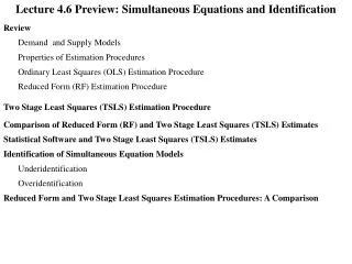
Lecture 4.6 Preview: Simultaneous Equations and Identification. Review. Demand and Supply Models. Properties of Estimation Procedures. Ordinary Least Squares (OLS) Estimation Procedure. Reduced Form (RF) Estimation Procedure. Two Stage Least Squares (TSLS) Estimation Procedure.

E N D
Lecture 4.6 Preview: Simultaneous Equations and Identification Review Demand and Supply Models Properties of Estimation Procedures Ordinary Least Squares (OLS) Estimation Procedure Reduced Form (RF) Estimation Procedure Two Stage Least Squares (TSLS) Estimation Procedure Comparison of Reduced Form (RF) and Two Stage Least Squares (TSLS) Estimates Statistical Software and Two Stage Least Squares (TSLS) Estimates Identification of Simultaneous Equation Models Underidentification Overidentification Reduced Form and Two Stage Least Squares Estimation Procedures: A Comparison
Review: Simultaneous Equation Demand and Supply Models Endogenous Variables: Qt and Pt Exogenous Variables: FeedPt and Inct Ordinary Least Squares (OLS) Estimation Procedure: Simultaneous Equation Problem Question: When an endogenous explanatory variables is present, is the ordinary least squares (OLS) estimation procedure for its coefficient value unbiased? No. consistent? No. PRS 1 Reduced Form (RF) Estimation Procedure Quantity Reduced form Equation: Price Reduced form Equation: 332.00 17.347 = 314.3 = 921.5 1.0562 .0108825 Question: When an endogenous explanatory variables is present, is the reduced form (RF) estimation procedure for its coefficient value PRS 2 No. Yes. unbiased? consistent?
Instrument Variable Estimation Procedure: A Review Instrument – Correlated Variable: Choose a variable that is correlated with the “problem” explanatory variable (the explanatory variable suffering from measurement error that creates the ordinary least squares (OLS) bias problem). Regression 1 Dependent Variable:“Problem” explanatory variable. Explanatory Variable: Instrument, the correlated variable. Regression 2 Dependent Variable: Original dependent variable Explanatory Variable:Estimate of the “problem” explanatory variable based on the results from Regression 1. Two Stage Least Squares (2SLS): An Instrumental Variable Two Step Approach – A Second Estimation Procedure 1st Stage: Estimate the variable that is creating the problem, the explanatory endogenous variable: Dependent variable: “Problem” explanatory variable. The endogenous explanatory variable in the original simultaneous equation model. The variable that creates the bias problem. Explanatory variables: All exogenous variables. 2nd Stage: Estimate the original models using the estimate of the “problem” explanatory endogenous variable Dependent variable: Original dependent variable. Explanatory variables: Estimate of the “problem” explanatory variable, the endogenous explanatory variable, based on the 1st stage and any relevant exogenous explanatory variables.
Endogenous Variables: Qt and Pt Exogenous Variables: FeedPt and Inct 1st Stage: Estimate the variable that is creating the problem, the explanatory endogenous variable: Dependent variable: “Problem” explanatory variable. The endogenous explanatory variable in the original simultaneous equation model. The variable that creates the bias problem. In this case, the price of beef, P, is the problem explanatory variable. Explanatory variables: All exogenous variables. In this case, the exogenous variables are FeedP and Inc. 1st Stage: Dependent variable: P Explanatory variables: FeedP and Inc Estimated Equation:EstP = 33.027 + 1.0562FeedP + .018825Inc
2nd Stage: Estimate the original models using the estimate of the “problem” explanatory endogenous variable Dependent variable: Original dependent variable. In this case, the original explanatory variable is the quantity of beef, Q. Explanatory variables: Estimate of the “problem” explanatory variable, the endogenous explanatory variable, based on the 1st stage and any relevant exogenous explanatory variables. 2nd Stage – Beef Market Demand Model: Dependent variable: Q Explanatory Variables: EstP and Inc Estimated Equation:EstQD = 149,107 314.3EstP + 23.26Inc 2nd Stage – Beef Market Supply Model: Dependent variable: Q Explanatory Variables: EstP and FeedP Estimated Equation:EstQS = 108,292 + 921.5EstP 1,305.2 FeedP
Reduced Form and Two Stage Least Squares Estimates: A Comparison Estimate Reduced Form (RF) Two Stage Least Squares (TSLS) 314.3 314.3 921.5 921.5 Two Stage Least Squares (TSLS) the Easy Way: Let EViews do the work: Highlight all relevant variables: Q P Inc FeedP Double Click, Click Options and then choose Two-Stage Least Squares Instrument List: The exogenous variables – IncFeedP Equation Specification: The dependent variable followed by the explanatory variables Demand Model: Q P Inc Supply Model: Q P FeedP
Reduced Form Estimation Procedure: Taking Stock Quantity Reduced Form Equation: EstQ = 38,726 332.00FeedP + 17.347Inc Price Reduced Form Equation: EstP = 33.027 + 1.0562FeedP + .018825Inc Suppose that FeedP increases while Inc remains constant: Suppose that Inc increases while FeedP remains constant: Does the demand curve shift? Yes Does the demand curve shift? No Does the supply curve shift? No Does the supply curve shift? Yes What happens to Q and P? What happens to Q and P? Q = 332.00FeedP Q = 17.347Inc P = 1.0562FeedP P = .018825Inc Price Price S’ S FeedP constantInc increases Inc constantFeedP increases D’ P = .018825Inc P = 1.0562FeedP S Q =17.347Inc Q = 332.00FeedP D D Quantity Quantity Q 332.00FeedP 332.00 Q 17.347Inc 17.347 = = = = 314.3 = = 921.5 P 1.0562FeedP 1.0562 P .018825Inc .018825 QD QS = = 314.3 = = 921.5 P P
Exogenous variables: FeedP and Inc. There are a total of 2 exogenous variables Price Price S’ S FeedP constantInc increases Inc constantFeedP increases D’ P = .018825Inc P = 1.0562FeedP S Q =17.347Inc Q = 332.00FeedP D D Quantity Quantity QD QS = = 314.3 = = 921.5 P P Demand Model Supply Model Changes in FeedP allows us to estimate demand model’s P coefficient Changes in Inc allows us to estimate supply model’s P coefficient Counting Counting Exogenous variable absent from the model Endogenous explanatory variable in the model Exogenous variable absent from the model Endogenous explanatory variable in the model 1 1 1 1 equals equals Critical role played by the absent exogenous variables.
Identification of Simultaneous Equation Models: Order Condition Number of exogenous variablesabsent from the model Less Than Number of endogenous explanatory variables in the model Equal To Greater Than ModelIdentified ModelOveridentified ModelUnderidentified No Estimates Unique Estimates Multiple Estimates
Underidentified Suppose that no income data were available? Simultaneous Equation Demand and Supply Models Endogenous Variables: Qt and Pt Exogenous Variables: FeedPt and Inct Quantity Reduced Form Equation: Dependent Variable: Q Explanatory Variables: FeedP Price Reduced Form Equation: Dependent Variable: P Explanatory Variables: FeedP
Quantity Reduced Form Equation: EstQ = 239,158 821.85FeedP Price Reduced Form Equation: EstP = 142.02 + .52464FeedP Suppose that FeedP increases while Inc remains constant: Suppose that Inc increases while FeedP remains constant: Does the demand curve shift? No Does the demand curve shift? Yes Does the supply curve shift? Yes Does the supply curve shift? No What happens to Q and P? What happens to Q and P? Q = 821.85 FeedP Q = ??????Inc P = .52464FeedP P = ??????Inc Price Price S’ S FeedP constantInc increases Inc constantFeedP increases D’ P = ??????Inc P = .52464FeedP S Q =??????Inc Q = 821.85FeedP D D Quantity Quantity Q 821.85 FeedP 821.85 Q ?????? Inc ?????? = = = = 1,566.5 = = ????? P .52464FeedP .52464 P ?????? Inc ?????? QD QS = = 1,566.5 = = ?????? P P
Exogenous variable: FeedP There is a total of 1 exogenous variable. Price Price S’ FeedP constantInc increases Inc constantFeedP increases D’ P = .52464FeedP S Q =821.85FeedP D D Quantity Quantity QD = = 314.3 P Demand Model Supply Model Changes in FeedP allows us to estimate demand model’s P coefficient Changes in Inc allows us to estimate supply model’s P coefficient Counting Counting Exogenous variable absent from the model Endogenous explanatory variable in the model Exogenous variable absent from the model Endogenous explanatory variable in the model 1 1 0 1 equals less than Critical role played by the absent exogenous variables.
Two Stage Least Squares (TSLS) Estimation Procedure Simultaneous Equation Demand and Supply Models Endogenous Variables: Qt and Pt Exogenous Variables: FeedPt and Inct Beef Market Demand Model: Dependent variable: Q Explanatory Variables: P and Inc Instrument List: FeedP = 1,566.5 Beef Market Supply Model: Dependent variable: Q Explanatory Variables: P and FeedP Instrument List: FeedP Error Message: Order condition violated.
Overidentified Suppose that the price of chicken is also available. Simultaneous Equation Demand and Supply Models Endogenous Variables: Qt and Pt Exogenous Variables: FeedPt, Inct, and ChickPt Quantity Reduced Form Equation: Dependent Variable: Q Explanatory Variables: FeedP, Inc, and ChickP Price Reduced Form Equation: Dependent Variable: P Explanatory Variables: FeedP, Inc, and ChickP
Quantity RF Equation: EstQ = 138,194 349.54FeedP + 16.865Inc + 47.600ChickP Price RF Equation: EstP = 29.962 + .95501FeedP + .016043Inc + .27464ChickP Suppose that FeedP increases while Inc and ChickP remains constant: Exogenous variables: FeedP, Inc, and ChickP A total of 3 exogenous variables Does the demand curve shift? No Does the supply curve shift? Yes What happens to Q and P? Demand Model Q = 349.54FeedP P = .95501FeedP Price Changes in FeedP allows us to estimate demand model’s P coefficient S’ Inc constant ChickP constantFeedP increases Counting Endogenous explanatory variable in the model Exogenous variable absent from the model P = .95501FeedP S Q = 49.54FeedP D 1 1 equals Quantity Q 349.54FeedP 349.54 Critical role played by the absent exogenous variables. = = = 366.0 P .95501FeedP .95501 QD = = 366.0 P
Quantity RF Equation: EstQ = 138,194 349.54FeedP + 16.865Inc + 47.600ChickP Price RF Equation: EstP = 29.962 + .95501FeedP + .016043Inc + .27464ChickP Suppose that Inc increases while FeedP and ChickP remain constant: Suppose that ChickP increases while FeedP and Inc remain constant: Does the demand curve shift? Yes Does the demand curve shift? Yes Does the supply curve shift? No Does the supply curve shift? No Q = 16.865Inc Q = 47.600ChickP P = .016043Inc P = .27464ChickP Price Price FeedP constantChickP constantInc increases FeedP constantInc constantChickP increases S S D’ D’ P = .016043Inc P = .27464Inc Q =16.865Inc Q =47.600Inc D D Quantity Quantity Q 16.865Inc 16.865 Q 47.600ChickP 47.600 = = = = 1,051.2 = = 173.3 P .016043Inc .016043 P .27464ChickP .27464 QS QS = = 1,051.2 = = 173.3 P P
Exogenous variables: FeedP, Inc, and ChickP There are 3 exogenous variables. Price Price FeedP constantChickP constantInc increases S FeedP constantInc constantChickP increases S D’ D’ P = .016043Inc P = .27464Inc Q =16.865Inc Q =47.600Inc D D Quantity Quantity QS QS = = 1,051.2 = = 173.3 P P Supply Model Changesin Inc allows us to estimate supply model’s P coefficient Changesin ChickP allows us to estimate supply model’s P coefficient Counting Exogenous variable absent from the model Endogenous explanatory variable in the model 1 2 greater than Critical role played by the absent exogenous variables.
Two Stage Least Squared Estimation Procedure = 366.0 = 893.5
Identification of Simultaneous Equation Models Number of exogenous variablesabsent from the model Less Than Number of endogenous explanatory variables in the model Equal To Greater Than ModelIdentified ModelOveridentified ModelUnderidentified No Estimates Unique Estimates Multiple Estimates Demand Model Number of exogenous variablesabsent from the model Number of endogenous explanatory variables in the model Exogenous Variables RF TSLS FeedP and Inc 1 1 314.3 314.3 FeedP 1 1 1,566.5 1,566.5 FeedP, Inc and, ChickP 1 1 366.0 366.0 Supply Model RF TSLS FeedP and Inc 1 1 921.5 921.5 FeedP 0 1 - - FeedP, Inc and, ChickP 2 1 1,051.2 173.3 893.5 Identified: Identical Overidentified: Reduced form provides multiple estimates. Underidentified: Identical Two stage least squares provides a single estimate.