Optimizing Transshipment and Minimum Cost Flow Problems with LP Formulations
430 likes | 556 Vues
This lecture covers the LP formulation of transshipment problems and minimum cost flow problems, focusing on decisions, constraints, and rationality in setting up the problems. The formulation of transshipment problems as transportation problems is also discussed, along with interpretations, capacitated versions, and examples. Lastly, it explores minimum cost flow problems with bounds and conversions from bounded to unbounded problems.

Optimizing Transshipment and Minimum Cost Flow Problems with LP Formulations
E N D
Presentation Transcript
Lecture 3 Transshipment ProblemsMinimum Cost Flow Problems 1
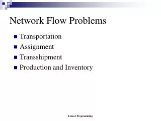
Agenda transshipment problems minimum cost flow problems 2
Transshipment Problems intermediate nodes C and D with flows passing through, neither created nor destroyed minimum cost flows to send the goods through the nodes C A G E F D B 20 3 60 7 5 4 2 45 9 1 40 8 11 6 35 4
LP Formulation of Transshipment Problems what are the decisions? let xij be the amount of flow from node i to node j objective: min 7xAC + 4xAD + 9xBC + 11xBD + 3xCE + 5xCF + 2xCG + xDE + 8xDF + 6xDG D E A G F B C 20 3 60 7 5 4 2 45 9 1 40 8 11 6 35 5
LP Formulation of Transshipment Problems what are the rationale to set constraints? non-negativity: xij 0 i, j phenomena to model related to the distribution of goods equivalent to a valid flow pattern D E A G B F C 20 3 60 7 5 4 2 45 9 1 40 8 11 6 35 每一個限制式都是用符號和數學關係表達一個物理現象。 6
LP Formulation of Transshipment Problems a valid flow pattern conservation of flows at all nodes node A: xAC + xAD = 60 node B: xBC + xBD = 9 node C: xAC + xBC = xCE + xCF + xCG node D: xAD + xBD = xDE + xDF + xDG node E: xCE + xDE = 20 node F: xCF + xDF = 45 node G: xCG + xDG = 35 D E A G B F C • min objective of a flow pattern, • s.t. conditions to be a flow pattern. 20 3 60 7 5 4 2 45 9 1 40 8 11 6 35 7
LP Formulation of Transshipment Problems min 7xAC + 4xAD + 9xBC + 11xBD + 3xCE + 5xCF + 2xCG + xDE + 8xDF + 6xDG s.t. node A: xAC + xAD = 60 node B: xBC + xBD = 9 node C: xAC + xBC = xCE + xCF + xCG node D: xAD + xBD = xDE + xDF + xDG node E: xCE + xDE = 20 node F: xCF + xDF = 45 node G: xCG + xDG = 35 xij 0 i, j E D C G F B A 20 3 60 7 5 4 2 45 9 1 40 8 11 6 35 8
Formulating a Transshipment Problem as a Transportation Problem motivation: simple solution method for transportation problems how to transform is node C (D)a source (i.e., a supplier)? a sink (i.e., a customer)? D E A G F B C 20 3 60 7 5 4 2 45 9 1 40 8 11 6 35 9
Formulating a Transshipment Problem as a Transportation Problem nodes C and D: both a source and a sink A E E D G D G F F B B C C A 20 3 D’ C’ 5 2 two linked transportation problems 45 1 20 3 8 60 7 5 6 4 2 35 45 9 1 0 40 8 11 6 60 7 35 4 0 9 40 11 10
Formulating a Transshipment Problem as a Transportation Problem unsure flows: 0 xCC’ 100, 0 xDD’ 100 11
Formulating a Transshipment Problem as a Transportation Problem observation: internal flow of zero cost does not affect the problem flow of 20 (or 2,000) units at no cost from node C to node C does not change the problem B G E D F C A 20 3 60 7 5 4 2 45 9 1 40 8 11 6 35 0 12 0
Formulating a Transshipment Problem as a Transportation Problem unsure flows: 0 xCC’ 100, 0 xDD’ 100 B E G D F C A 20 3 60 7 5 4 2 45 9 1 40 8 11 6 100 35 100 13 100 100
unsure flows: 0 xCC’ 100, 0 xDD’ 100 Formulating a Transshipment Problem as a Transportation Problem G B B E D D G E D F F C C A A C 20 60 7 20 4 3 60 7 45 5 4 2 40 9 45 11 9 1 35 40 8 11 3 5 6 100 100 2 100 0 35 100 6 8 1 100 100 0 14 100 100
interpretation of the flow pattern, e.g., Formulating a Transshipment Problem as a Transportation Problem G B B E D D E G F D F C C A A C 20 60 20 20 60 60 60 45 20 45 40 45 45 30 30 25 10 35 40 10 100 25 100 10 35 10 100 100 90 10 15
Capacitated Transshipment Problems lower and upper bounds for xij 0 ≤ lij ≤ xij ≤ uij any algorithms solving transshipment problems can solve the capacitated version of a transshipment problem 16
Exercise Model the problem as a balanced transportation problem G A D E B F C 20 3 60 7 5 4 2 45 2 9 1 40 8 11 6 35 17
Minimum Cost Flow Problems A = the set of assignment problems T = the set of transportation problems TS = the set of transshsipment problems MCF = the set of minimum cost flow problems A T TS MCF 19
Minimum Cost Flow Problems balanced flow directed arcs an undirected arc replaced by two directed arcs with opposite directions 20
Example 5.4 of [7] min 5x02+4x13+2x23+6x24+5x25+x34+2x37 +4x42+6x45+3x46+4x76, s.t. a constraint for a node, based on conservation of flow 22
Minimum Cost Flow Problems special structure optimal integral solution if all availabilities, requirements, and capacities being integral solution methods: linear programming (i.e., Simplex), transportation Simplex, network flow methods 23
Minimum Cost Flow Problems with Bounds two general approaches to solve lij xij uij either algorithms specially for bounded MCF problems or converting a bounded MCF problem to an unbounded one 24
Converting a Bounded MCF to an Unbounded One what does the paragraph mean? if you don’t know what to do, work with a simple numerical example. 25
Minimum Cost Flow c01 = 3, c02 = 1, c12 = 2 inflow of node 0 = 8 outflow of node 2 = 8 MCF = ? all 8 units through (0, 2), of cost 8 1 2 0 2 3 8 8 1 26
Relaxing a Lower Bound MCF: all 8 units through (0, 2), of cost 8 suppose 5 x01 how to convert the problem into an unbounded MCF problem? 1 2 0 2 3 8 8 1 27
Relaxing a Lower Bound LP formulation 1 2 0 2 3 8 8 1 28
Relaxing a Lower Bound define y01 = x01-5 1 2 0 2 3 8 8 1 29
How Does the Network Look Like? an unbounded network 1 2 0 5 2 3 3 8 1 30
Relaxing the Lower Bound l01 = 5 objective function changed to min 3y01+2x12+x02+15 question: is it possible to convert to a network of the objective function without adding 15 by oneself? 0 2 1 1 2 0 5 2 3 2 3 3 8 8 8 1 1 31
Relaxing the Lower Bound l01 = 5 how about adding a dummy node a such that c0a = 3, ca1 = 0, outflow from a = 5 adding a dummy inflow of 5 to node 1 2 1 0 0 2 1 2 1 0 a 5 5 5 2 3 2 3 3 8 8 8 2 0 3 1 1 8 8 1 32
Relaxing an Upper Bound MCF: all 8 units through (0, 2), of cost 8 suppose x02 7 how to convert the problem into an unbounded MCF problem? 1 2 0 2 3 8 8 1 33
Relaxing an Upper Bound suppose x02 7 0 2 1 1 2 a 0 2 3 8 8 1 2 3 8 8 1 0 7 7 34
Negative Cost? possible to have negative cost as long as there is no negative cost cycle e.g., if c24 = -6 35
Generalization of MCF from one commodity (i.e., product) to multi-commodity (i.e., multiple products) flow without gain to with gain 36
Multi-Commodity Flow Problems two types of products 1 2 0 (cij, uij): (cost, upper bound) of an arc (2, 4) (3, 4) type 1: 5 type 1: 5 (1, 6) type 2: 3 type 2: 3 37
Multi-Commodity Flow Problems “An extension of the problem of finding the minimum cost flow of a single commodity through a network is the problem of minimizing the cost of the flows of several commodities through a network. This is the minimum cost multi-commodity network flow problem. There will be capacity limitations on the flows of individual commodities through certain arcs as well as capacity limitations on the total flow of all commodities through individual arcs.” … “The resultant model has a block angular structure of the type discussed in Section 4.1.” 38
LP Formulation of a Two-Commodity Flow Problem let xij be the flow of type 1 commodity along arc (i, j) let yij be the flow of type 1 commodity along arc (i, j) 1 2 0 (2, 4) (3, 4) type 1: 5 type 1: 5 (1, 6) type 2: 3 type 2: 3 39
LP Formulation of a Two-Commodity Flow Problem “The resultant model has a block angular structure of the type discussed in Section 4.1.” 1 2 0 (2, 4) (3, 4) type 1: 5 type 1: 5 (1, 6) type 2: 3 type 2: 3 40
LP Formulation of a Two-Commodity Flow Problem 1 2 0 (2, 4) (3, 4) type 1: 5 type 1: 5 (1, 6) type 2: 3 type 2: 3 objective function flowconservation of type 1 product flowconservation of type 2 product arc capacity constraints 41
Network Flow with Gains Model flows not conserved x units into arc (i, j), ijx units out of node j, ij 1 solved by integer programming if integral values required 42