Discrete-Time Convolution and FIR Filters Overview
210 likes | 273 Vues
Understand the concept of convolution in discrete time systems and the implementation of FIR filters. Explore properties and applications with examples.

Discrete-Time Convolution and FIR Filters Overview
E N D
Presentation Transcript
Signals and Systems Fall 2019 Discrete-Time Convolution and Filtering Concept Prof. Dr. Adnan Kavak Computer Engineering Kocaeli University Textbook: Linear Systems and Signals, B.P. Lathi These slides are used in EE313 course at the University of Texas at Austin. They are adopted in this course with Courtesy of Prof. Brian L. Evans
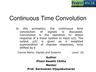
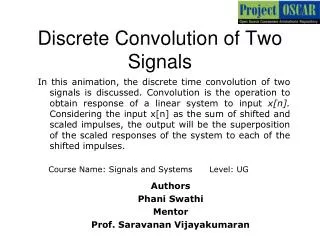
Discrete-time convolution For every value of n, we compute a new summation Continuous-time convolution For every value of t, we compute a new integral x[n] h[n] y[n] x(t) h(t) y(t) LTI systemrepresentedby its impulseresponse LTI system representedby its impulseresponse Discrete-Time Convolution
Unit Impulse Response • Discrete-time unit impulse signal d[n] d[n] d[n-2] 1 1 n n -3 -2 -1 0 1 2 3 -3 -2 -1 0 1 2 3 • Expressing finite-length signals using unit impulses x[n] 3 d[n] 3 n = -3 : 3; x = [0 1 2 3 2 1 0]; stem(n, x); 2 d[n+1] 2 d[n-1] 2 d[n-2] d[n+2] 1 - OR - n = -3 : 3; x = 3*tripuls(n/6); stem(n, x); n -3 -2 -1 0 1 2 3 No MATLAB function for d[n] Could use rectpuls(n) but awkward
d[n] T{•} h[n] Unit Impulse Response • Output of system when unit impulse d[n] is input • When system is a finite impulse response filter • Impulse responses for 3-point and 7-point averaging filters M = 2; n = -2 : 10; h = rectpuls((n-1) / 3); h = h / (M+1); stem(n, h); ylim( [0, 0.5] ); M = 6; n = -2 : 10; h = rectpuls((n-M/2) / (M+1)); h = h / (M+1); stem(n, h); ylim( [0, 0.5] ); n n
Discrete-time Convolution Preview Block Diagram Representations
Discrete-Time Convolution Preview • Assuming that h[n] has finiteduration from n = 0, …, N-1 • Block diagram of an implementation of a finite impulse response(FIR) digital filter: flip and slide x[n] z-1 z-1 … z-1 … h[0] h[1] h[2] h[N-1] S y[n]
Convolution and FIR Filters • FIR filters of order M Input-output relationship: • Impulse response h[n] = bn for 0 ≤ n ≤ M • Called a finite convolution sum • Output y[n] obtained by convolvingx[n] and h[n] • Convolution • Input-output algorithm for large class of filters including FIR • Applies to infinite-length signals • More on general case later
Computing Discrete Time Convolution • Expand finite convolution sum 3 x[n] h[n] 2 1 1 n n -3 -2 -1 1 2 3 4 5 2 3 4 -1 0 y[n]is one sample longer than x[n] x = [1 2 3]; h = [1 -1]; y = conv(x, h); - OR - x = [1 2 3 0]; h = [1 -1]; y = filter(h, 1, x);
h[n] Averaging filter impulse response n 0 1 2 3 Computing Discrete Time Convolution • Impulse response h[n] has extent 0 ≤ n ≤ M • Example: Two-point averaging filter M = 1 y[n] = h[0] x[n] + h[1] x[n-1] = ( x[n] + x[n-1] ) / 2 h = [1 1]; x = [0 1 2 3 2 1 0]; y = conv(h, x); • Discrete-time convolution demos • http://spfirst.gatech.edu/matlab/#dconvdemo • http://pages.jh.edu/~signals/discreteconv2/index.html
Discrete Time Convolution Properties • Output y[n] for inputx[n] • Decompose x[n] into weighted sum of delayed impulses • Apply additivity • Apply homogeneity • Apply time-invariance • Apply change of variables
Convolution Properties • Convolution with impulse • Commutative property Showed this earlier on slide 8-7 • Associative property Non-zero when m = n – n0
Cascaded LTI Systems • Switching the order of cascaded LTI systems Application of associative property of convolution
Running-Average Filter • Filter alters input Removes component or modifies characteristic coffee filter[Wikipedia] • Finite impulse response (FIR) filter • Each output sample is finite sum of weighted input samples • Running-average (a.k.a. moving average) filter • Each output sample is average of finite number of input samples • Example:y[n] = ( x[n] + x[n+1] + x[n+2] ) / 3 sliding window x[n] y[n] 6 6 4 4 2 n n -3 -2 -1 1 2 3 4 5 6 7 -3 -2 -1 1 2 3 4 5 6 7 0 0
Running-Average Filter • Noncausal filter Uses future input values (as in example on previous slide) Buffer input signal before computing nth output sample • Causal filter • Only uses present and past input values • Compute nth output sample when nth input sample arrives • Example: y[n] = ( x[n] + x[n-1] + x[n-2] ) / 3 sliding window x[n] y[n] 6 6 4 4 2 n n -3 -2 -1 1 2 3 4 5 6 7 -3 -2 -1 1 2 3 4 5 6 7 0 0
General FIR Filter • Causal FIR filter Sliding window of M+1 samples M+1 filter coefficients b0, b1, …, bM Vector dot product of [b0b1 … bM] and [x[n] x[n-1] … x[n-M]] • Averaging filter • Three terms: filter order M = 2 and bk = 1/3 for k = 0, 1, 2 • General case: bk = 1/(M+1) for k = 0, 1, …, M • Coefficients completely define filter • Example: { bk } = { 1, -1 } gives y[n] = x[n] – x[n-1] • Example: { bk } = { 1, 0, -1 } gives y[n] = x[n] – x[n-2]
FIR Filtering • Signal is sum of increasing exponential & sinusoid x[n] = (1.02)n+ ½ cos((2 p / 8)n + p / 4) for 0 ≤ n ≤ 40 • Apply causal 3-point and 7-point averaging filters b = { bk } = { 1/3, 1/3, 1/3 } where M = 2 b = { bk } = { 1/7, 1/7, 1/7, 1/7, 1/7, 1/7, 1/7 } where M = 6 n n n
FIR Filtering (MATLAB Code) % Define x[n] for 0<=n<=40 n = 0 : 40; x1 = (1.02).^n; x2 = 0.5*cos((2*pi/8)*n + pi/4); x = x1 + x2; % Save n and x1 for plotting trend t = n; x1t = x1; % Define x[n] for -6<=n<=50 n0 = 6; n = [ (-n0:-1) n (41:50) ]; x = [ zeros(1,n0) x zeros(1,10) ]; x1 = [ zeros(1,n0) x1 zeros(1,10) ]; % Define filter coefficients b3coeff = (1/3)*ones(1,3); b7coeff = (1/7)*ones(1,7); % Filter data y3 = filter(b3coeff, 1, x); y7 = filter(b7coeff, 1, x); % Plot results figure; stem(n, x); title('x[n]'); ylim([0 3]); hold on; plot(t, x1t); hold off; figure; stem(n, y3); title('Output of 3-Point Filter'); ylim([0 3]); hold on; plot(t, x1t); hold off; figure; stem(n, y7); title('Output of 7-Point Filter'); ylim([0 3]); hold on; plot(t, x1t); hold off; Note:filter(b, 1, x) command Input signal Filter coefficients
Audio Example • Signal is sum of three B notes on Western scale Where fB6 = 1975.53 Hz, fB4 = 493.883 Hz, fB2 = 123.471 Hz With sampling rate fs = 8000 Hz and Note:fB6 = ¼ fB4 and fB4 = ¼ fB2 due to octave spacing • Filter signal with 4-point averaging filter • b = { bk } = { 1/3, 1/3, 1/3 } where M = 2 • Filter signal with 16-point averaging filter • b = { bk } = { 1/16, 1/16, 1/16, …, 1/16 } where M = 15 • What differences do you hear?
Audio Example (MATLAB code) % Set sampling rate andduration fs = 8000; tmax = 3; nmax = round(fs * tmax); n = 1 : nmax; % E note in threedifferentoctaves B6 = 1975.53; % Hz B4 = B6/4; B2 = B4/4; f = [ B6 B4 B2 ]; wHat = 2*pi*f/fs; a = [ 1 1 1 ]; x = zeros(1, length(n)); for i = 1 : length(wHat) x = x + a(i)*cos(wHat(i)*n); end % Scale amplitude to be in [-1, 1] x = x / max(abs(x)); % Filter signal of 3 notes average4 = (1/4)*ones(1,4); y4 = filter(average4, 1, x); average16 = (1/16)*ones(1,16); y16 = filter(average16, 1, x); % Play soundstokeepsamevolumelevel soundsc(x, fs); pause(tmax+1); soundsc(y4, fs); pause(tmax+1); soundsc(y16, fs); Note:filter(b, 1, x) command Input signal Filter coefficients