Aggregate Expenditure Model
Aggregate Expenditure Model. Overview. With this section we begin to build a model of the economy. Early on our focus will be on answering a few basic questions: 1) What determines the level of RGDP?, and 2) Why does RGDP go up and down over time?


Aggregate Expenditure Model
E N D
Presentation Transcript
Overview With this section we begin to build a model of the economy. Early on our focus will be on answering a few basic questions: 1) What determines the level of RGDP?, and 2) Why does RGDP go up and down over time? Some guy named John Maynard Keynes (rhymes with rains, like in the southern plains – Keynes is a peculiar spelling to us, ain’t it? Keynesian is pronounced by saying Keynes Ian real fast – please do not say Ka knee sion), was one of the first folks to work out this model. Others have tinkered with it since the mid-1930’s.
Overview Keynes felt that in the short run the price level in the economy was fixed. Producers will supply all that demanders want, without changes in the price level. We will build a model of RGDP in this section based on this idea. In the chapter it might seem that we are talking about GDP. But in a time of no price level change, GDP = RGDP.
Basic idea The amount of goods and services produced (and therefore the level of employment) depend directly on the level of total aggregate expenditure. Aggregate expenditure represents the spending plans of the players of the economic game. We assume for now we have only two players, households and businesses. Household expenditures are called consumption expenditures(C) and business expenditures are called investment expenditures(I). Note the book has a subscript g on I. I will not type it to save time and space.
Key point of our theory Aggregate expenditure will be C + I and these terms represent plans. GDP will be measured on the horizontal axis and the 45 degree line will translate the GDP to a vertical distance. You recall from the actual measurement we have GDP = C + I. These actual measurements are just labeled GDP. We will play a scenario analysis and just pick a GDP level. At that GDP level we will compare the actual C and actual I that result with what has been planned.
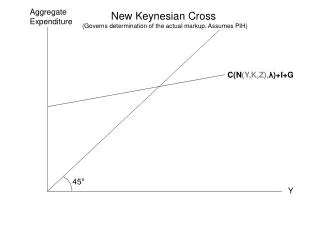
Graph we use The level of output in the economy will be where the C+I line crosses the 450 line. The only way output can change in our model is if C or I should change. C, I 450 C+I C output GDP1 To fully understand this theory we need to 1) understand the mechanics of this graph 2) Understand why we look at where C+I crosses the 450 line 3) see why C and I combined appear this way in the graph.
mechanics C, I 450 If you just focus your eyes of the 450 line you could note a square. The nice thing about a square is that the length of the bottom equals the length of the height. C+I C { output { GDP1 We want to train our eyes to first consider a level of output along the horizontal axis and compare that output with the level of C+I. But C+I is measured vertically. The level of output can be converted to a vertical distance by thinking of the box height.
practice C, I 450 AT the level of output shown, which is greater, output or C+I? C+I C output GDP Remember to translate the output to the height of the box and that really is the height of the 450 line.
practice again C, I 450 AT the level of output shown, which is greater, output or C+I? C+I C output GDP
practice one more time C, I 450 C+I AT the level of output shown, which is greater, output or C+I? C output GDP
C again Recall that C stands for household consumption and we said it is a plan by households to consume at various levels of income given 2) the wealth of households 3) expectations, 4) real interest rates, 5) Household debt, 6) taxation. Note this about the model: If we think about any GDP level the C line tells us what consumers plan to spend. Then when a GDP level actually happens the actual consumption will be the amount on the C line above the GDP level. In other words the planned consumption always equals the actual consumption.
I again Recall that I stands for business investment and we said it is a plan by businesses at various levels of income given 1) Acquisition, maintenance, and operating costs, 2) Business taxes, 3) technological change, 4) stock of capital goods on hand, and 5) expectations, and 6) the interest rate. Note 2 things here: i) investment is constant at various GDP levels, and ii) investment is different from C in a fundamental way. Business have to think about how much C will be and they have to plan their own investment which includes how much to put in inventory.
More I again If businesses miscalculate C the amount that ends in inventory will be different than what businesses plan and this will cause them to change the amount of output they make. We will see this real soon, I just want to tip you off to be on the lookout for it. On the next slide you see how I add the constant amount I onto the C line to get C + I. Most of the time we will skip putting in the I line by itself.
C+I C+I Putting the C and I lines together means at each output level add up C and I. Note if C or I should change, the C+I line will shift. C } I } C I
Equilibrium Before I mentioned we need to understand why we look at where C+I crosses the 450 line to get the GDP level in the economy. The reason is based on producers of output wanting their inventory to be at the ‘right’ level. If producers (businesses) find that inventories are being depleted more than they want, they will produce more goods and services to get the inventory to the level they desire. GDP would rise. If producers find that inventories are being accumulated more than they want, they will produce less goods and services to get the inventory to the level they desire. GDP would fall.
equilibrium In the graph we had before the height of the 450 line represents the level of output produced. This production would include what firms feel they need to produce to make inventory what they want. The C+I line indicates how much goods and services households and businesses want to buy. If C+I is greater than the output produced then inventories must be depleted more than business want and thus output is expanded. If C+I is less than the output produced then inventories must be accumulating more than business want and thus output is lowered.
disequilibrium C, I 450 AT the level of output shown, which is greater, output or C+I? C+I C output GDP Since C+I is greater than the output, inventories must be falling and production will be increased. In our theory the output shown couldn’t exist for long given the C+I plans of households and businesses. So at the current time the level of output shown is ruled out as the current level of output.
disequilibrium again C, I 450 AT the level of output shown, which is greater, output or C+I? C+I C output GDP Since C+I is less than the output, inventories must be rising and production will be decreased. In our theory the output shown couldn’t exist for long given the C+I plans of households and businesses. So at the current time the level of output shown is ruled out as the current level of output.
Equilibrium C, I 450 C+I AT the level of output shown, which is greater, output or C+I? C output GDP In this diagram at the output level shown C+I = output and firms have no reason to change production because inventories are at the right level.
Change in Equilibrium If households or businesses change their expenditure plans, then the C+I line will shift and the level of output will change. The output change is the same if we have a shift of the C line or the I line in the same amount.
Change in investment C, I Say the economy has C1+I1 and the resulting GDP1. Now if the interest rate should fall investment would rise to, say I2. The result would be C1+I2 and GDP2. GDP increases because with the additional I inventories C1+I2 C1+I1 GDP GDP1 GDP2 would be too low and thus production, and hence GDP, would increase.
Change in investment C, I Now we want to note the change in GDP is greater than the change in investment. The change in investment is the vertical shift of the C+I line and the change in GDP is the horizontal change from GDP1 to GDP2. C1+I2 C1+I1 A B D GDP GDP1 GDP2 The idea that the change in GDP is greater than the shift in the curve is the multiplier. We saw this already!
The multiplier In the graph on the previous slide I should probably have the C + I be steeper than what I have. For most of what I want to communicate the graph is fine. But here it is misleading. Note when investment goes up GDP rises. The GDP rise can be seen as either distance increase D or distance A + B. Since we move to points on the 45degree line A + B = D. Now A is the initial change in investment. The B is all the rounds of addition consumption that result from A. D is a multiple of A, as we saw before.
Government In our model the government can have an impact on the economy in two ways: 1) by affecting expenditures directly by its own expenditures, what will be called G, 2) by changing taxes and thus changing consumption C. Government expenditure in this model will not depend on the level of GDP, but instead depend on the political process. Thus G will look much like I in the model and can change if done so in the political arena. Remember if taxes change by some amount w, C changes in the opposite direction by MPC times w.
RGDP graph G In the RGDP diagram the level of G will not depend on the level of RGDP. In this regard it is similar to investment. The level of G can shift up or down, as we will see shortly. G1 RGDP
RGDP graph C, I, G The expenditure line is now the C+I+G line and the equilibrium level of RGDP occurs where the C+I+G line cross the 45 degree line as we said in the past. C1+I1+G1 G1 RGDP
example C, I, G Say the government decides to spend more. If the MPC = .8, how much does RGDP rise? C1+I1+G2 C1+I1+G1 RGDP RGDP1 RGDP2
Tax change X Say the government decides to tax less. If the MPC = .8, how much does RGDP rise? C2+I1+G1 C1+I1+G1 RGDP RGDP1 RGDP2 This answer to this question requires some thought. Let’s do some of this. More on the next screen.
Tax change A change in the level of taxation has an impact on the consumption of the household. If taxes change by a dollar, for example, the income households have to dispose of would really change by a dollar. Before we saw if income changed by a dollar then consumption would change by the MPC. So a change in the level of taxes will change consumption by MPC times the change taxes.
review In general the change in RGDP = 1 initial change in spending. 1 - MPC Now the initial change in spending could be from a change in 1) C, but not due to a change in tax, 2) I, 3) G If there is a change in the tax level use the change in the tax level as the initial change in spending, but also put minus the MPC into the numerator of the bracketed term to incorporate the impact the tax change has on the level of consumption.
Sneaky example If the government increased expenditure by 10 the C+I+G+X line would shift up by 10. If at the same time they increased taxes by 10 and the MPC was .9 the C+I+G+X line would fall by ...........................? If we put the two together at the same time, what is called a balanced budget change(not a balanced budget), the C+I+G+X line would shift on the net.................. and the total change in income would be....................? So the balance budget change leads to RGDP increasing by the amount of the G change.
Exports and imports At this time we want to incorporate the foreign sector into the model. This means we need to incorporate exports and imports. Remember imports need to be incorporated because C, I and G include imported items. By the way when we have both government and net exports in the model we have “open, mixed – economy” model. Open means international segment is included and mixed means we have government sector included.
exports X The amount of net export is not dependent on our level of RGDP. Other countries decide to buy our stuff. In our model net exports is a constant much like G and I. If they decide to buy more the line shifts up. X RGDP RGDP1 RGDP2
RGDP graph C, I, G, X C1+I1+G1 +X1 The expenditure line is now the C+I+G+x-M line and the equilibrium level of RGDP occurs where the C+I+G+X-M line cross the 45 degree line as we said in the past. X RGDP
RGDP graph C, I, G, X C1+I1+G1 +X2 C1+I1+G1 +X1 RGDP If the mpc = .8 and net exports rises by 100, the change in income (100)/(1 - .8) = 500.
Changes in net exports The net export amount can change and if so the component X will change causing the whole C + I + G + X line to shift. Net exports can change if 1) Foreign economies have income growth (X rises) or decline (X falls). The idea is the amount they buy from us varies with their. The more income the more of our stuff they buy.
Summary AE AE2 Aggregate Expenditure AE = C + I + G + X. We see the level of RGDP is determined by AE. If AE changes RGDP will change. AE1 RGDP RGDP1 RGDP2 The mechanism for change will be that inventories are not at the planned level and thus output will be changed to meet those plans.
Gaps AE Keynes felt the economy was guided by AE. But, he also felt the resultant RGDP level may or may not occur at full employment in the economy. AE1 RGDP RGDP1 So, Keynes recognized if RGDP is not at the full employment level of RGDP (the potential of the economy) then we had a problem. Let’s see these ideas next.
Look at that gap in the dudes teeth. You probably see the gap as a horizontal space. Recessionary GAP AE The recessionary gap here is a vertical space Here full employment RGDP is above RGDP1 . The economy will stay at RGDP1 because of AE1. The problem is then that resources are left unused. AE1 RGDP Full employment RGDP RGDP1 Note the recessionary gap is a vertical distance and is the amount by which AE is too low to have full employment RGDP.
Inflationary Gap AE Here the actual level of output is above full employment. The problem here is that eventually there will be inflationary pressure. AE1 Inflationary Gap RGDP Full employment RGDP RGDP1 The inflationary gap is the vertical distance by which AE is too high above the level that is needed to have full employment.