Brian Mapes MPO seminar September 26, 2012

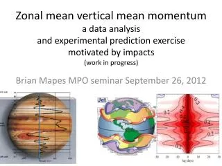
1. Zonal mean vertical mean momentuma data analysis and experimental prediction exercisemotivated by impacts(work in progress) Brian Mapes MPO seminar September 26, 2012

2. Outline • Motivation: impacts on our latitude (25N) • Background: • an old planetary physics problem • meaningful vs. arbitrary averaging • Time series at one latitude • A full latitude-time analysis • climatology • anomalies and their budgets • Statistical prediction of anomalies by LIM • Conclusions

3. Barotropic zonal mean flow and TCs High-Low tercile <[u]>20-30°N composite (ASO) iBTracs data

4. H500 H

5. Zonal mean "pushes" the subtropical highs(by exerting a PV tendency) Heating (PV source) Eddy Z1000 no [u] Eddy Z1000 w/ July [u] Chen, Hoerling & Dole 2001

6. Barotropic zonal mean flow and TCs High-Low tercile <[u]>20-30°N composite (ASO)

7. Outline • Motivation: impacts on our latitude (25N) • Background: • an old planetary physics problem • meaningful vs. arbitrary averaging • Time series at one latitude • A full latitude-time analysis • climatology • anomalies and their budgets • Statistical prediction of anomalies by LIM • Conclusions

9. Basic u equation • use x,y instead of lon,lat for clarity • phyd coordinate in vertical (no rclutter) • "usual approximations" (no f*w) Convergence of 3D flux (by both fluid and molecular motions) Cor PGF

10. Break flux into components • and group d/dx terms: • Zonal average on a phydsurface is []: p surface H L H L "mountain torque"

11. Mass-weighted vertical average <> • These 4 (+1) terms must add up (physics)... • But in data (reanalysis-estimated budgets) there is a 6th (implied) term: "residual" Friction Net Coriolis transport (meridionallyacross latitude lines) + + mtn torque + TENDENCY = it is small

12. "Meaningful" averaging and <[u]> • The averaged quantity <[u]>obeys an equation w/ fewer, smaller, & simpler terms than u • It is thus "harder to change" than local u, so it has an existence (and, we will see, a persisence) that is arguably more substantial than u • This is quite unlike many averages of many quantities that we sum up in our computers! • many are just fictions or conveniences • to blend (but dilute) information or signals, or reduce "noise" • I'll speak of <[u]> as a wind that "advects" scalars

13. <[u]>, GLobal AAM and length of day • Velocity * lever arm *circumference of lat line • GLAAM = <[u]> (a cos(f)) (2p a cos(f)) • GLAAM exchanged w/ solid Earth (conserved)  measurable length of day fluctuations • semiannual, ENSO, MJO • (much <[u]> lit. as AAM)

14. Zonal mean vs. “Annular modes” • NAM or “Arctic Oscillation” are EOFsof SLP • Related to NAO = pAzores-pIceland • decomposition debate: semantic? profound? • NAM/SAM are patterns w/ max SLP’2 (variance) • averaged over polar cap surface area • Some link to <[u]> via geostrophy, but loose • Example of arbitrary vs. meaningful averaging • SLP’2 does not obey a physics equation that area-averaging interestingly refines • If we end up calling it ‘annular’, why not use annuli? []

15. Outline • Motivation: impacts on our latitude (25N) • Background: • an old planetary physics problem • meaningful vs. arbitrary averaging • Global picture  Time series at 25N • A full latitude-time analysis • climatology • anomalies and their budgets • Statistical prediction of anomalies by LIM • Conclusions

16. Data used • NCEP-NCAR Reanalysis ("NCEP1") • 1980-2011 (32 years) • 94 equally spaced latitudes (~2o, "Gaussian") • Courtesy Dr. Klaus Weickman (NOAA PSD) who computed the zonal means and budget terms • for his papers over ~20 years • in spherical, sigma coordinates rather than p • (MERRA used for some climatology figs)

17. textbook: 4 jets, with meanders

18. <[u]> u200annual mean [u200] anncyc Jan -------------------------- Dec

19. climatology of <[u]> Annual mean map MERRA 1000-100 mb MERRA 1000-100 mb NCEP1 sigma 1-21 NCEP1 all levels 45 30 30 45 All Scales: +/- 25 m/s

20. u 50 mb annual mean and cycle

21. Outline • Motivation: impacts on our latitude (26N) • Background: • an old planetary physics problem • meaningless vs. meaningful averaging • Time series at our latitude (26N) • A full latitude-time analysis • climatology • anomalies and their budgets • Statistical prediction of anomalies by LIM • Conclusions

22. <[u]> at 26N

23. data => mean clim(doy) + anomaly(doy,y) color = year (blue  red rainbow)

24. data => mean clim(doy) + anomaly(doy,y)

25. data => mean clim(doy) + anomaly(poy,y)

26. Quantify seasonality: RMS (or stdev) • Winter has bigger anomalies on average than summer • anomalies are strongly persistent from day to day • (5-day data pre-averaging doesn’t reduce their square very much) • (the heavy line) ?

27. Winter anomalies are bigger • Midwinter (ground hog day) minimum?

28. Winter anomalies are bigger • Midwinter (ground hog day) minimum?

29. Quantify longevity of anomaliesby lagged multiplication

30. Quantify longevity by lagged multiplication 1980 mean of all years 1983

31. Quantify longevity by lagged multiplication Repeat for all 30 days in March Mean of all March 1s mean of all March days' means over all years Mean of all March 31s

32. Quantify longevity by lagged multiplication Repeat for all months of the year Magnitude difference is distracting. We already quantified that winter anomalies are larger: the lag-0 variance. So divide by that to normalize. (this is "auto-covariance") Feb Jan Mar mean of all months Dec Summer

33. Quantify longevity by lagged multiplication Repeat for all months of the year Feb Mar Jan Apr Dec mean acov of all months normalized by its lag=0 value May Feb Jan Mar mean acov of all months Dec Summer

34. Repeat for all months of the year Feb Mar Jan Apr Sep Dec characteristic lifetime (2/a) ~25 d Oct JJA May Nov IDEA: is it exponential decay C=C0 exp(-t/15d)? ... a solution of this ...  (univariate) ? both ...a postulatedreinterpretation of:

35. data => mean clim(doy) + anomaly(doy,y)

36. Power = | FT(autocov) |2 broad hump @ "wave period" ~2 characteristic times (50d) 2 Period (months)

37. Histogram of 26N <[u]> anomalies INCONSISTENT w/ this univariate model, at least w/Gaussian, white noise (Ornstein-Uhlenbeck process)

39. Outline • Background: an old planetary physics problem • Motivation: impacts on our latitude • Our time series (26N) • A full latitude-time analysis • climatology • anomalies • Statistical prediction of anomalies by LIM • Outstanding questions

40. climatology of <[u]> Annual mean map MERRA 1000-100 mb MERRA 1000-100 mb NCEP1 sigma 1-21 NCEP1 all levels 45 30 30 45 All Scales: +/- 25 m/s

41. Real time monitoring (Klaus Weickmann) 25N 2011 2012 MAY SEP JAN http://www.esrl.noaa.gov/psd/map/clim/aam.rean.shtml

42. Characterize timescale w/autocorr.

43. autocov(lag,lat) = autocorr(lag,lat)*stdev2(lat)

44. autocov(lag,lat) = autocorr(lag,lat)*stdev2(lat)

45. <[u]> anomalies are more persistenton edges of jets Annual mean map MERRA 1000-100 mb 45 45 Jan  Dec

46. Timescale: extend this to lag x lat 1980 mean of all years 1983

47. Composite anomalies in lag x latweighted by 26N base time series etc. etc. for 32 years (optionally for seasons) and sum it all up *apply with pos. weight *apply with negtive weight

48. This weighted composite is an array of regression coefficients (slopes of linear fits onbase(t) vs. field(t+lag,lat) scatterplots at each altitude) "Characteristic" time scales AND latitude evolution same, along base lat... All seasons:

49. Can do the same for tendency field, and torques m/s composite of d/dt = d/dt(composite)

50. TRANSPORT (FRICTION) Budget(composite over anomalies in all seasons) MTN RESIDUAL TEND TEND = MTN + TRANSPORT + (FRICTION+GW) + CORIOLIS + RESIDUAL