Download
1 / 75
1.21k likes | 2.41k Vues
Grain Boundary Engineering & Coincident Site Lattice (CSL) Theory. Texture, Microstructure & Anisotropy A.D. Rollett. Last revised: 18 th Mar. ‘14. Objectives. The objectives of this lecture are: Develop an understanding of grain boundary engineering

E N D
Grain Boundary Engineering& Coincident Site Lattice (CSL) Theory Texture, Microstructure & Anisotropy A.D. Rollett Last revised:18thMar. ‘14
Objectives • The objectives of this lecture are: • Develop an understanding of grain boundary engineering • Explain the theory of Coincident Site Lattices (CSLs) and how it applies to grain boundaries • Show how microstructures are analyzed for CSL content
References • Interfaces in Crystalline Materials, Sutton & Balluffi, Oxford U.P., 1998. Very complete compendium on interfaces. • Interfaces in Materials, J. Howe, Wiley, 1999. Useful general text at the upper undergraduate/graduate level. • Crystal Defects and Crystalline Interfaces, W. Bollmann, (1970). New York, Springer Verlag. • Grain Boundary Migration in Metals, G. Gottstein and L. Shvindlerman, CRC Press, 1999. The most complete review on grain boundary migration and mobility. • Materials Interfaces: Atomic-Level Structure & Properties, D. Wolf & S. Yip, Chapman & Hall, 1992. • Bollmann, W. (1982), Crystal lattices, interfaces, matrices. Published by the author, Geneva. • Grimmer, H., Disorientations and coincidence rotations for cubic lattices. ActaCrystall. A30 (1974) 685–688. • Grimmer, H., Bollmann, W., Warrington, D. H., Coincidence- site lattices and complete pattern-shift lattices in cubic crystals. ActaCryst. A30 (1974) 197 – 207. • Bonnet, R., et al. (1981). Determination of near-Coincident Cells Hexagonal Crystals - Related DSC Lattices. ActaCrystall. A37 184-189. • Ikuhara, Y. and P. Pirouz (1996). Orientation relationship in large mismatched bicrystals and coincidence of reciprocal lattice points (CRLP). In: Intergranular and Interphase Boundaries in Materials, Pt 1. 207 121-124.
Outline • Slides from Integran with examples of Grain Boundary Engineered materials • CSL theory • Brandon’s criterion for classification of grain boundaries by CSL type • Technical information on comparative properties of GBE and non-GBE materials
Reading • Pages 3-25 of Sutton & Balluffi • Pages 307-346 of Howe.
Grain Boundary Engineering • Grain Boundary Engineering (GBE) is the practice of obtaining microstructures with a high fraction of boundaries with desirable properties. • In general, desirable properties are associated with boundaries that have simple, low energy structures. • Such low energy structures are, in turn, associated with CSL boundaries. • GBE generally consists of repeated cycles of deformation and annealing, chosen so as to generate large fractions of “special boundaries” and avoid development of strong recrystallization textures. • GBE is largely confined at present to fcc metallic systems such as stainless steel, nickel alloys, Pb, Cu. • Note that detailed information on exactly which CSL boundaries have useful properties is lacking, as is information on how the typical processing routes actually produce high fractions of CSL boundaries.
Courtesy of: Metallurgical Nano-Technology Grain boundary engineering (GBE™) is the methodology by which the local grain boundary structure is characterized and material processing variables adjusted to create an optimized grain boundary microstructure for improved material performance. Nanocrystalline materialsare those in which the average crystal size is reduced 1000-fold from the micron-range in conventional materials to the nanometer size range (3-100nm). This can be cost -effectively achieved by proprietary electrodeposition techniques (NanoPlate™).
GBE Surface Treatment Alloy 625 GBE Technology Grain boundary engineering (GBE™) is the methodology by which the local grain boundary structure is characterized and material processing variables adjusted to create an optimized grain boundary microstructure for improved material performance. Base Material • Patent-Protected Thermo-Mechanical Metallurgical Process • Applied during component forming/fabrication processes. Can also be applied as a surface treatment (0.1 to 1mm) to finished or semi-finished structures. • Increases Population of ‘Special’ Grain Boundaries • Reduces Average Grain Size • Enhances Microstructural Uniformity • Fully Randomizes Crystallographic Texture Special GB’s (red;yellow) General GB’s(black) Integran’s GBE technology has also been applied to mitigate stress corrosion cracking susceptibility of Ni-base alloys, extend the service-life of lead-acid battery grids, and improve the fatigue and creep performance of aerospace superalloys.
Conventional(fsp<15%) after 2 weeks of cycling. GBE(fsp=55%) after 4 weeks of cycling. Lead-Acid Batteries Integran’s innovative GBE® grid processing technology is designed to extend the service life of conventional SLI and industrial batteries (US Patent No. 6,342,110 B1). The cycle - life of lead-acid batteries (e.g., automotive) is compromised by intergranular degradation processes (corrosion, cracking). Palumbo, G. et al. (1998). "Applications for grain boundary engineered materials." Journal of Minerals, Metallurgy and Materials (JOM)5040-43. Conventional lead-acid battery grid (Pb-1wt%Sb) following 4 years of service.
Corrosion of Aluminum 2124 • Results from experiment involving intergranular corrosion of aluminum alloy 2124. Low angle boundaries are measurably more resistant than high angle boundaries. Some evidence for resistance of 3 and 7 boundaries (possibly also 3). Research by Lisa Chan, CMU.
Corrosion in Ni Alloy 600 (Ni-base alloy) Several 3 boundaries with larger deviations from ideal misorientation cracked. Gertsman et al., Acta Mater., 49 (9): 1589-1598 (2001).
S3 Boundaries Ni3Al Cracked 3 boundaries were found to deviate more than 5°from the trace of the {111} plane. Lin et al., Acta Metall. Mater., 41 (2): 553-562 (1993). 13
R o o m T e m p e r a t u r e F a t i g u e P e r f o r m a n c e o f S e l e c t e d N i c k e l B a s e d A l l o y s 1 2 0 0 0 0 0 C o n v e n t i o n a l 1 0 0 0 0 0 0 G B E Cycles to Failure 8 0 0 0 0 0 6 0 0 0 0 0 4 0 0 0 0 0 2 0 0 0 0 0 0 A l l o y 6 2 5 / 6 0 k s i A l l o y 7 3 8 / 4 0 k s i V 5 7 / 4 0 k s i M a t e r i a l / S t r e s s Fatigue
Conventional GBE Creep Thaveeprungsriporn, V. and G. S. Was (1997). "The role of coincidence-site-lattice boundaries in creep of Ni-16Cr-9Fe at 360 degrees C." Metallurgical And Materials Transactions A 28(10): 2101; Alexandreanu, B. et al. (2003). "The effect of grain boundary character distribution on the high temperature deformation behavior of Ni-16Cr-9Fe alloys." Actamaterialia51 3831. Alloy V57 Alloy 625
Special Grain Boundaries • There are some boundaries that have special properties, e.g. low energy. • In most known cases (but not all!), these boundaries are also special with respect to their crystallography. • When a finite fraction of lattice sites coincide between the two lattices, then one can define a coincident site lattice (CSL). • A boundary that contains a high density of lattice points in a CSL is expected to have low energy because of good atomic fit. • Note that the boundary plane matters, in addition to the misorientation; this means, in effect, that only pure tilt or pure twist boundaries are likely to have a high density of CSL lattice points. • Relevant website: http://www.tf.uni-kiel.de/matwis/amat/def_en/kap_7/illustr/a7_1_1.html (a page from a general set of pages on defects in crystals: http://www.tf.uni-kiel.de/matwis/amat/def_en/index.html ).
Grain Boundary properties S3 60°<111> • For example,fcc <110> tilt boundaries show pronounced minima in energy • However, some caution needed because the <100> series do not show these minima. S11 50°<110> Figure taken from Gottstein & Shvindlerman, based on Goux, C. (1974). “Structure des joints de grains: consideration cristallographiques et methodes de calcul des structures.” Canadian Metallurgical Quarterly13: 9-31.]
Kronberg & Wilson • Kronberg & Wilson in 1947 considered coincidence patterns for atoms in the boundary planes (as opposed to the coincidence of lattice sites). Their atomic coincidence patterns for 22° and 38° rotations on the 111 plane correspond to the S13b and S7 CSL boundary types. Note the significance of coincidence in the plane of the boundary. • Friedel also explored CSL-like structures in a study of twins. Kronberg, M. L. and F. H. Wilson (1949), “Secondary recrystallization in copper”, Trans. Met. Soc. AIME, 185, 501-514 (1947). Friedel, G. (1926). Lecons de Cristallographie (2nd ed.). Blanchard, Paris.
Sigma=5, 36.9° <100> [Sutton & Balluffi]
CSL = geometrical concept • The CSL is a geometrical construction based on the geometry of the lattice. • Lattices cannot actually overlap! • If a (fixed) fraction of lattice sites are coincident, then the expectation is that the boundary structure will be more regular than a general boundary. • Atomic positions are not accounted for in CSLs. • It is possible to compute the density of coincident sites in the plane of the boundary - this goes beyond The basic CSL concept, which has to do only with the lattice misorientation.
CSL construction • The rotation of the second lattice is limited to those values that bring a (lattice) point into coincidence with a different point in the first lattice. • The geometry is such that the rotated point (in the rotated lattice 2) and the superimposed point (in the fixed lattice 1) are related by a mirror plane in the unrotated state.
Rotation to Coincidence • Red and Green lattices coincide Points to be brought into coincidence
S5 relationship Red and Green lattices coincide after rotation of 2 tan-1 (1/3) = 36.9°
Rotation to achieve coincidence [Bollmann, W. (1970). Crystal Defects and Crystalline Interfaces. New York, Springer Verlag.] • Rotate lattice 1 until a lattice point in lattice 1 coincides with a lattice point in lattice 2. • Clear that a higher density of points observed for low index axis.
CSL rotation angle y • The angle of rotation can be determined from the lattice geometry. The discrete nature of the lattice means that the angle is always determined as follows.q = 2 tan-1 (y/x),where (x,y) are the coordinates of the superimposed point (in 1); x is measured parallel to the mirror plane. x
CSL <-> Rodrigues • You can immediately relate the angle to a Rodrigues vector because the tangent of the semi-angle of rotation must be rational (a fraction, y/x); thus the magnitude of the corresponding Rodrigues vector must also be rational! • Example: for the S5 relationship, x=3 and y=1; thus q = 2 tan-1 (y/x) = 2 tan-1 (1/3) = 36.9° and the rotation axis is [1,0,0], so the complete Rodrigues vector = [1/3, 0, 0].
The Sigma value (S) • Define a quantity, S', as the ratio between the area enclosed by a unit cell of the coincidence sites, and the standard unit cell. For the cubic case that whenever an even number is obtained for S', there is a coincidence lattice site in the center of the cell which then means that the true area ratio, S, is half of the apparent quantity. Therefore S is always odd in the cubic system.
Generating function • Start with a square lattice. Assign the coordinates of the coincident points as (n,m)*: the new unit cell for the coincidence site lattice is square, each side is √(m2+n2) long. Thus the area of the cell is m2+n2. Correct for m2+n2 even: there is another lattice point in the center of the cell thereby dividing the area by two. • * n and m are identical to xand y discussed in previous slides
Range of m,n • Restrict the range of mand nsuch that m<n. • If n=m then all points coincide, and m>ndoes not produce any new lattices. • Example of 5: m=1, n=3, area =(32+12) = 10; two lattice points per cell, therefore volume ratio = 1:5; rotation angle =2 tan-11/3 = 36.9°. m n
Generating function, contd. • Generating function: we call the calculation of the area a generating function. Sigma denotes the ratio of the volume of coincidence site lattice to the regular lattice
Generating function: Rodrigues • A rational Rodrigues vector can be generated by the following expression, where {m,n,h,k,l} are all integers, m<n.r= m/n [h,k,l] • The rotation angle is then: tan q/2 = m/n√(h2+k2+l2)
Sigma Values • A further useful relationship for CSLs is that for sigma. Consider the rotation in the (100) plane:tan{q/2} = m/n • area of CSL cell = m2+n2= n2 (1 + (m/n)2) = n2 (1 + tan2{q/2}) • Extending this to the general case, we can write:S = n2 (1 + tan2{q/2}) =n2(1 + {m/n√(h2+k2+l2)}2) = n2 + m2(h2+k2+l2) • Note that although using these formulas and inserting low order integers generates most of the low order CSLs, one must go to values of n~5 to obtain a complete list. [Ranganathan, S. (1966). “On the geometry of coincidence-site lattices.” ActaCrystallographica21197-199; see also the Morawiec book, pp 142-149 for discussion of cubic and lower symmetry cases]
Quaternions • Recall that all CSL relationships can be thought of as twin relationships, which means that (in a centrosymmetric lattice) they can be constructed as 180° rotations about some axis. • Rotations of 180° have a very simple representation as a quaternion (by contrast to Rodrigues vectors) because cos(q/2)=cos(90°)=0 and sin(90°)=1. Therefore for a rotation axis of [x,y,z] the unit quaternion = {x,y,z,0}. • Take the S5 as an example. The rotation axis is [310], therefore the quaternion representation is 1/√10{3,1,0,0}. • Check that this is indeed the expected value by applying symmetry to the ∆g and indeed one finds that this is equivalent to {1/3,0,0} as a Rodrigues vector or 38.9°[100]. • One can further check that a vector of type [310] is mapped onto its negative by using the quaternion to transform/rotate it. If we choose [-1,3,0] as being orthogonal to the [310] access, we can use the standard formula. PTO…
Quaternions, contd. • Note that q0 = 0 in these cases (of 180° rotations) and q2=1, so that simplifies the formula considerably:s = -v + 2(v•q) q= -v+ 2(v•[310]) [310] • Pick [-1,3,0] as an example:= -v+ 2([-1,3,0]•[3,1,0]) [3,1,0]= -v+ 2([-3+3+0]) [3,1,0]= [+1,-3,0] • Note that any value of the z coefficient will also satisfy the relationship. • Note that any combination of b=-3a in [a,b,c] (i.e. that has integer coordinates to be a point in the lattice, and is perpendicular to the axis) will also work. This helps to make the point that there is an infinite set of points that coincide, each of which satisfies the required relationship. That infinite set of coincident points is the Coincident Site Lattice.
Table of CSL values in axis/angle, Euler angles, Rodrigues vectorsand quaternions Note: in order to compare a measured misorientation with one of these values, it is necessary to compute the values to high precision (because most are fractions based on integers). Note: integer fractions are quoted for most of the Rodrigues vectors. The entries in decimals also correspond to integer values and will be updated at a later time.
CSL + boundary plane • Good atomic fit at an interface is expected for boundaries that intersect a high density of (coincident site) lattice points. • How to determine these planes for a given CSL type? • The coincident lattice is aligned such that one of its axes is parallel to the misorientation axis. Therefore there are two obvious choices of boundary plane to maximize the density of CSL lattice points:(a) a pure twist boundary with a normal // misorientation axis is one example, e.g. (100) for any <100>-based CSL; (b) a symmetric tilt boundary that lies perpendicular to the axis and that bisects the rotation should also contain a high density of points. Example: for S5, 36.9° about <001>, x=3, y=1, and so the (310) plane corresponds to the S5 symmetric tilt boundary plane [i.e. (n,m,0)].
CSL boundaries and RF space • The coordinates of nearly all the low-sigma CSLs are distributed along low index directions, i.e. <100>, <110> and <111>. Thus nearly all the CSL boundary types are located on the edges of the space and are therefore easily located. • There are some CSLs on the 210, 331 and 221 directions, which are shown in the interior of the space.
RF pyramid and CSL locations R1+R2+R3=1 l =111 l =100 (√2-1,√2-1) (√2-1,0) l =110
Plan View:Projection on R3= 0 <110>,<111> 33c <111> linelies over the <110> line <100>
Fractions of CSL Boundaries in a Randomly Oriented Microstructure • It is interesting is to ask what fraction of boundaries correspond to each sigma value in a randomly oriented polycrystal? • The method to calculate such (area) fractions is exactly the same as for volume fractions in an Orientation Distribution. • The Brandon Criterion establishes the “capture radius” for each sigma value (which decreases with increasing sigma value). • All points (in a discretized MD) are assigned to a given CSL type if they fall within the capture radius.
CSL % for Random Texture Garbaczet al., Scr. Mater., 23 (8): 1369-1374 (1989). Gertsmanet al., Acta Metall. Mater., 42 (6): 1785-1804 (1994). Morawiecet. al., Acta Metall. Mater., 41 (10): 2825-2832 (1993). Pan et al., Scr. Metall. Mater., 30 (8): 1055-1060 (1994). Generate MD from a random texture; analyze for fraction near each CSL type (method to be discussed later).
Grain Boundaries from High Energy Diffraction Microscopy Measurements made at the Advanced Photon Source: see Hefferanet al. (2009). CMC 14 209-219. Pure Nickel: 42 layers, 4 micron spacing, 0.16 mm3 Pure Ni sample, 42 layers3,496 grains; ~ 23,598 GBs