Waveform Inversion Techniques for High-Resolution Crosswell Data Analysis
This study from the University of Utah's Geology and Geophysics Department explores the use of waveform inversion for crosswell data, aiming to achieve high-resolution imaging of subsurface structures. The presentation covers key motivations, objectives, theoretical frameworks, and presents synthetic model examples. The results indicate that higher resolution tomograms exhibit greater sensitivity to initial models, offering improved insights into lithological variations at a resolution of 2m by 2m. Conclusions emphasize the potential for future applications and testing on 2-D field data.

Waveform Inversion Techniques for High-Resolution Crosswell Data Analysis
E N D
Presentation Transcript
Waveform Inversion for Crosswell Data M. Zhou Geology and Geophysics Department University of Utah
Outline • Motivation • Objective • Theory • Examples • Synthetic Model 1 • Synthetic Model 2 • Conclusions
Motivation • High resolution 2 m by 2 m • Analyses of lithology
Outline • Motivation • Objective • Theory • Examples • Synthetic Model 1 • Synthetic Model 2 • Conclusions
Objective • High resolution tomogram
fast, insensitive to initial model low resolution (high freq. approx.) high resolution slow, sensitive to initial model Traveltime vs. Waveform • Traveltime Inversion • Waveform Inversion
Traveltime • Waveform • Initial model • High resolution Objective • + • provide initil model
Outline • Motivation • Objective • Theory • Examples • Synthetic Model 1 • Synthetic Model 2 • Conclusions
D s(x) b(x,t) | t=0 f(x,t) Gradient Forward field Residual backward field Theory Waveform inversion: Misfit = S (dobs-dcal(s))2 Residual waveform = *
Outline • Motivation • Objective • Theory • Examples • Synthetic Model 1 • Synthetic Model 2 • Conclusions
X (m) 0 50 km/s 0 6.0 5.0 40 Depth (m) 4.0 3.0 80 Model Model 1: Model 1m X 1m grid 41 shots/geophones 200 Hz Ricker wavelet Shortest wavelength 20 m
X (m) X (m) X (m) 0 0 0 50 50 50 km/s 0 6.0 5.0 40 Depth (m) 4.0 3.0 80 WI50 Model Tomo50 (ray-based) Model 1: Tomograms
X (m) X (m) X (m) 0 0 0 50 50 50 km/s 0 6.0 5.0 40 Depth (m) 4.0 3.0 80 WIF30 + WI20 Model WIF30 Model 1: Tomograms
X (m) X (m) X (m) 0 0 0 40 40 40 80 80 80 0 Time (sec) 0.1 Tomo50 (ray-based) Model WIF30 + WI20 Model 1: Synthetic CSG
Time (s) Time (s) .01 .01 .04 .04 .025 .025 1. Amplitude 0. -1. Ray-based Traveltime Inversion WIF30 1. Amplitude 0. -1. WI50 WIF30 + WI20 Model 1: One trace
Outline • Motivation • Objective • Theory • Examples • Synthetic Model 1 • Synthetic Model 2 • Conclusions
X (m) 0 90 km/s 0 3.6 3.2 100 Depth (m) 2.8 2.4 210 Model Model 2: Model 3m X 3m grid 18 shots / 32 geophones 60 Hz Ricker wavelet
X (m) X (m) X (m) 0 0 0 90 90 90 km/s 0 3.6 3.2 100 Depth (m) 2.8 2.4 210 WIF20 Model WT10 (wave eq.) Model 2: Tomograms
X (m) X (m) X (m) 0 0 0 90 90 90 km/s 0 3.6 3.2 100 Depth (m) 2.8 2.4 210 WIF20 + WI10 Model WIF20 Model 2: Tomograms
X (m) X (m) 0 0 0 100 100 100 200 200 200 X (m) 0 0.1 Time (sec) WT10 Model WIF20 Model 2: Synthetic CSG
Time (s) .04 .12 .08 1. Amplitude 0. -1. Wave Eq. Traveltime (WT) 10 iterations 1. Amplitude 0. -1. WIF20 Model 2: One Trace
Outline • Motivation • Objective • Theory • Examples • Synthetic Model 1 • Synthetic Model 2 • Conclusions
WI vs. Traveltime Inversion: WIF + WI vs. WI: Conclusions • Higher resolution tomograms; • More sensitive to initial model. • Less sensitive to initial model.
Future Work • Test on 2-D field data
Acknowledgements • I am grateful for the financial • support from the members of • the 2001 UTAM consortium.