Download
1 / 67
770 likes | 1.57k Vues
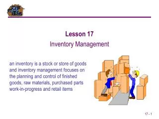
Lesson 17 Inventory Management. an inventory is a stock or store of goods and inventory management focuses on the planning and control of finished goods, raw materials, purchased parts work-in-progress and retail items. Independent Demand. Dependent Demand. A. C(2). B(4). D(2). E(1).

E N D
Lesson 17 Inventory Management an inventory is a stock or store of goods and inventory management focuses on the planning and control of finished goods, raw materials, purchased parts work-in-progress and retail items
Independent Demand Dependent Demand A C(2) B(4) D(2) E(1) D(3) F(2) Independent demand is uncertainDependent demand is certain
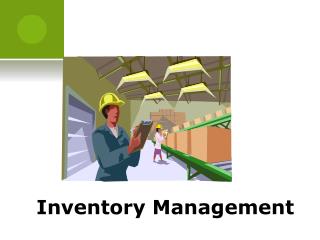
Different Types Of Inventory Inventory must be managed at various locations in the production process. .Rawmaterials or purchasedparts . Partially completed goods, called “work-in-progress (WIP)” .Finishedgoods inventories (manufacturing organizations) .Merchandise (retail organizations) .Replacement parts, tools and supplies .Goods-in-transit between locations (either plants, warehouses, or customers)
Work center Work center Work center Inventory Management Locations Production Process Work center WIP WIP Raw Materials Receiving Finished Goods
Functions Of Inventory Control Inventory control is necessary to . Meet anticipated demand . Smooth production requirements . De-couple components of the production-distribution system . Protect against stock outs . Take advantage of order cycles . Hedge against price increases or quantity discounts . Permit operations to function smoothly and efficiently . Increase cash flow and profitability The inventory manager is constantly striving to manage inventory to the right level. If you have too much then you are taking away from your cash flow. If you have too little you may not be running your operations smoothly and efficiently and disappointing your customers.
Some Terminology Some terms that common to inventory management are: . Lead time - time interval between ordering and receiving the order . Carrying (holding) cost - the cost of holding an item for a specified period of time (usually a year), including cost of money, taxes, insurance, warehousing costs, etc . Ordering costs - costs of ordering and receiving inventory . Shortage costs - costs resulting when demand exceeds the supply of inventory on hand often resulting in down time, unsatisfied customers, and unrealized profits . Cycle counting - a periodic physical count of a classification of inventory or selected inventory items to eliminate discrepancies between the physical count and the inventory management system
Objectives Of Inventory Control There are many objectives of inventory control. Simplistically they are to have the right amount (not too much – not too little) at the right place at the right time to maximize your cash flow, to have smooth efficient operations and to meet customer expectations. . Inventory is money! Inventories must be managed “cost effectively" giving consideration to .. Cost of ordering and maintaining inventory .. Carrying costs .. Timing of inventory to allow for smooth operations . Inventory is necessary to meet customer requirements. Inventory must be managed to a required level of customer service .. Ensure that the right product is produced at the right time to meet customer demand
Inventory Control Effectiveness There are several measurements to determine how well a company manages its inventory. Industry information and specific competitor information can be obtained though industry associations and published financial reports. .Days of inventory on hand - the amount of inventory on hand based on the expected amount of days of sales that can be supplied from the inventory .Inventory turnover - the ratio of annual cost of goods sold to average inventory investment .Customer satisfaction - quantity of backorders, percent of orders filled on time, customer complaints about delivery
Requirements For Effective Management Some of the requirements for effective inventory management include: . A system to keep track of the inventory on hand (raw materials, work-in-progress, finished goods, spare parts, etc). . A system to manage purchase orders . A reliableforecast of demand that includes the possible forecast error . Knowledge of leadtimes and leadtimevariability . Reasonable estimates of inventory holding costs, ordering costs, and shortage costs . A classification system for inventory items Integrated Management Information Systems are critical to the successful inventory manager. The inventory management system must be integrated with the financial, production,and customer service functions of the company.
Inventory Counting Systems Inventory is such a major factor in a business operations that Counting Systems are necessary to ensure that inventory is being managed properly. Inventory systems are only as good as the information they contain … and transaction errors can be very costly. . Periodic system - physical counts made at periodic intervals throughout the year . Perpetual (continual) inventory systems - keep track of additions and removals from inventory so that a continual running total of inventory on hand is available Most inventory systems today utilize “bar codes” to accurately track inventory movements easily and cost effectively. . Grocery stores . Retail stores . Auto rentals
Classification Systems The ABC method provides for classification of inventory according to some measure of importance (usually by annual dollar usage) A - very important (accuracy within .2 percent) B - moderately important (accuracy within 1 percent) C - least important (accuracy within 5 percent) The classification system does not necessarily mean that B and C items are unimportant from a production point of view. A stock-out of nuts and bolts which may be classified as C items can just as easily shut down a production line as a major component. High A Annual $ volume of items B C Low Few Many Number of Items
ABC Classification - Example Example 1: Classify the inventory items below as A, B or C.
How Much? When! How Much? When? To Order How much and when to order depends on many factors including: ordering costs, carrying costs, lead times, variability in lead times, variability in demand, variability in production, etc.. The Economic Order Quantity(EOQ) is the order size (how much?) that minimizes the total cost of inventory. The Reorder Point(ROP) is the inventory point (when?) which triggers a reorder.
How Much? How Much? To Order – EOQ Models There are 3 Economic Order Quantity (EOQ) models which can be used to determine how much to order. Each has a scenario under which it is appropriate. They are: . Basic EOQ – instantaneous delivery . EOQ – non-instantaneous delivery . EOQ – quantity discount
Q Usage/demand rate Reorder point Time Place order Place order Receive order Receive order Receive order Lead time Inventory Cycle – Instantaneous Delivery Inventory instantaneously increases by the quantity (Q) received. Quantity on hand Time
Basic EOQ – Instantaneous Delivery Model The Basic Economic Order– instantaneous delivery model assumptions are as follows: . Only one product is involved . Demand requirements are known . Demand is reasonably constant . Lead time does not vary . Each order is received in a single delivery (“instantaneously”) . There are no quantity discounts
Basic EOQ – Carrying Cost Carrying Cost Annual Carrying Cost is linearly related to the Order Quantity Order Quantity (Q)
Basic EOQ – Ordering Cost Ordering Cost Ordering Cost decreases as Order Quantity increases; however not linearly Order Quantity (Q)
Basic EOQ – Total Cost Total Cost Order Quantity (Q)
Basic EOQ – Instantaneous Delivery The Basic Economic Order– instantaneous delivery modelEOQ is the quantity which minimizes Total Cost = Carrying Cost + Ordering Cost. It is where Carrying Cost = Order Cost and is calculated by: Total Cost Basic EOQ
Basic EOQ – Example Example 2a: A local distributor for a national tire company expects to sell 9,600 steel belted radial tires of a certain size and tread design next year. Annual Carrying Cost is $16 per tire, and Ordering Cost is $75. The distributor operates 288 days per year. What is the EOQ?
Basic EOQ – Example Example 2b: How many times per year does the tire distributor reorder tires? Example 2c: What is the length of the order cycle (Cycle Time)?
Basic EOQ – Example Example 2d: What is the Total Annual Cost if the EOQ is ordered?
Basic EOQ – Example Example 3a: Piddling Manufacturing assembles security monitors. It purchases 3,600 black and white cathode ray tubes (CRT’s) at $65 each. Ordering costs are $31, and annual carrying costs are 20% of the purchase price. Compute the optimal order quantity.
Basic EOQ – Example Example 3b: Compute the total annual ordering cost for the optimal order quantity.
EOQ – Non-instantaneous Delivery Model The basic EOQ model assumes instantaneous delivery; however, many times an organization produces items to be used in the assembly of products. In this case the organization is both a producer and user. Orders for items may be replenished (non-instantaneously) over time rather than instantaneously.
EOQ – Non-instantaneous Delivery Model Consider the situation where a toy manufacturer makes dump trucks. . The manufacturer also produces (production rate) the rubber wheels that are used in the assembly of the dump trucks. Let’s consider 500 per day for example. . In this case the ordering costs associated with an order for rubber wheels would be the cost associated with the setup and delivery of the rubber wheels to the dump truck assembly area. . The manufacturer makes the dump trucks at constant rate per day (production rate). Let’s consider 200 per day for example. The inventory picture in this case is much different from the “saw-tooth” pattern we saw in the instantaneous model as shown on the next slide.
EOQ – Non-instantaneous Delivery Model As you see in this example, the inventory (shown in yellow) depends on the production rate (shown in blue) and the usage rate (shown in pink). How much to order depends on setup costs and carrying costs. The Economic Order Quantity(EOQ) is the order size that minimizes the total cost of inventory. Sometimes this is referred to as the EconomicRunQuantity because it is dependent on the cumulative manufacturing production quantity. Total cost = Carrying costs + Setup costs. A schematic of the non-instantaneous considerations are shown on the next slide.
Production/Usage Usage Only (EOQ - Run Size) Maximum Inventory Cumulative Production Amount on hand EOQ – Non-instantaneous Delivery Model
Non-instantaneous - Example Example 4a: A toy manufacturer uses 48,000 rubber wheels per year for its popular dump truck series. The firm makes its own wheels, which it can produce at a rate of 800 per day. The toy trucks are assembled uniformly over the entire year. Carrying cost is $1 per wheel per year. Setup cost for a production run of wheels is $45. The firm operates 240 days per year. Determine the optimal run size.
Non-instantaneous - Example Example 4b: Compute the minimum total cost for carrying and setup.
Non-instantaneous - Example Example 4c: Compute the cycle time for the optimal run size. Example 4d: Compute the run time for the optimal run size.
EOQ With Quantity Discount EOQ with Quantity Discount is very important because price reductions are frequently offered to induce customers to order in larger quantities. Why do you think this is done? In this model the purchasing cost will vary depending on the quantity purchased. Purchasing cost was omitted in the previous EOQ models because the price per unit was the same for all units; thus, the inclusion of the purchase cost would only increase the total cost function by the purchase cost amount. Thus, it would have had no effect on the EOQ calculation. This is illustrated in the next slide.
Adding Purchasing costw/o quantity discount doesn’t change EOQ TC with Purchasing Cost TC without Purchasing Cost Cost Purchasing Cost – same for all units Quantity EOQ EOQ Without Quantity Discount
EOQ With Quantity Discount In this model, how much to order depends on purchasecosts, setup costs and carrying costs. The Economic Order Quantity(EOQ) is the order size that minimizes the total cost of inventory. Sometimes this is referred to as the EconomicRunQuantity because it is dependent on the cumulative manufacturing production quantity. Total cost = Carrying costs + Ordering costs + Purchasing Cost
EOQ With Quantity Discount The Method of Computing EOQ with Quantity Discount is a step wise process. .First, compute the common EOQ using the earlier formula .Second, .. Identify the price range where the common EOQ lies .. If the common EOQ is in the lowest quantity range then the EOQ with quantity discount is the common EOQ .. Otherwise, the EOQ with quantity discount is the quantity where the total cost is minimum when considering the cost for the common EOQ and the cost for all minimum quantities of price breaks greater than the common EOQ.
EOQ With Quantity Discount - Example Example 5a: The maintenance department of a large hospital uses 816 cases of liquid cleanser annually. Ordering costs are $12, carrying costs are $4 per case per year, and the price schedule for ordering is listed below. Determine the optimal order quantity and the total cost. There are 240 days in a year.
Common EOQ = 70 Is in the second price break EOQ With Quantity Discount - Example
Common EOQ = 70 Is in the second price break EOQ With Quantity Discount - Example Therefore; the EOQ with quantity discount = minimum (TC(70), TC (80), TC (100))
EOQ With Quantity Discount - Example Therefore; the total cost is minimum for an order quantity of 100 and the EOQ with quantity discount = 100