Automatic Image Alignment Techniques in Computational Photography
This presentation delves into the methodologies for automatically aligning images, highlighting two primary approaches: feature-based and direct pixel-based alignment. The feature-based approach identifies matching features across images, while direct alignment uses brute force to maximize pixel agreement. The discussion addresses challenges with brute force methods, like computational inefficiency, and introduces advanced techniques such as pyramid search and gradient descent for optimizing alignment. Applications like motion estimation, image stabilization, and 3D reconstruction are also explored.


Automatic Image Alignment Techniques in Computational Photography
E N D
Presentation Transcript
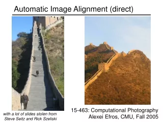
Automatic Image Alignment (direct) 15-463: Computational Photography Alexei Efros, CMU, Fall 2006 with a lot of slides stolen from Steve Seitz and Rick Szeliski
Image Alignment • How do we align two images automatically? • Two broad approaches: • Feature-based alignment • Find a few matching features in both images • compute alignment • Direct (pixel-based) alignment • Search for alignment where most pixels agree
Direct Alignment • The simplest approach is a brute force search (hw1) • Need to define image matching function • SSD, Normalized Correlation, edge matching, etc. • Search over all parameters within a reasonable range: • e.g. for translation: • for tx=x0:step:x1, • for ty=y0:step:y1, • compare image1(x,y) to image2(x+tx,y+ty) • end; • end; • Need to pick correct x0,x1 and step • What happens if step is too large?
Direct Alignment (brute force) • What if we want to search for more complicated transformation, e.g. homography? for a=a0:astep:a1, for b=b0:bstep:b1, for c=c0:cstep:c1, for d=d0:dstep:d1, for e=e0:estep:e1, for f=f0:fstep:f1, for g=g0:gstep:g1, for h=h0:hstep:h1, compare image1 to H(image2) end; end; end; end; end; end; end; end;
Problems with brute force • Not realistic • Search in O(N8) is problematic • Not clear how to set starting/stopping value and step • What can we do? • Use pyramid search to limit starting/stopping/step values • For special cases (rotational panoramas), can reduce search slightly to O(N4): • H = K1R1R2-1K2-1 (4 DOF: f and rotation) • Alternative: gradient decent on the error function • i.e. how do I tweak my current estimate to make the SSD error go down? • Can do sub-pixel accuracy • BIG assumption? • Images are already almost aligned (<2 pixels difference!) • Can improve with pyramid • Same tool as in motion estimation
Motion estimation: Optical flow Will start by estimating motion of each pixel separately Then will consider motion of entire image
Why estimate motion? • Lots of uses • Track object behavior • Correct for camera jitter (stabilization) • Align images (mosaics) • 3D shape reconstruction • Special effects
Key assumptions • color constancy: a point in H looks the same in I • For grayscale images, this is brightness constancy • small motion: points do not move very far • This is called the optical flow problem Problem definition: optical flow • How to estimate pixel motion from image H to image I? • Solve pixel correspondence problem • given a pixel in H, look for nearby pixels of the same color in I
Optical flow constraints (grayscale images) • Let’s look at these constraints more closely • brightness constancy: Q: what’s the equation? • small motion: (u and v are less than 1 pixel) • suppose we take the Taylor series expansion of I:
Optical flow equation • Combining these two equations • In the limit as u and v go to zero, this becomes exact
Optical flow equation • Q: how many unknowns and equations per pixel? • Intuitively, what does this constraint mean? • The component of the flow in the gradient direction is determined • The component of the flow parallel to an edge is unknown • This explains the Barber Pole illusion • http://www.sandlotscience.com/Ambiguous/barberpole.htm
Solving the aperture problem • How to get more equations for a pixel? • Basic idea: impose additional constraints • most common is to assume that the flow field is smooth locally • one method: pretend the pixel’s neighbors have the same (u,v) • If we use a 5x5 window, that gives us 25 equations per pixel!
RGB version • How to get more equations for a pixel? • Basic idea: impose additional constraints • most common is to assume that the flow field is smooth locally • one method: pretend the pixel’s neighbors have the same (u,v) • If we use a 5x5 window, that gives us 25*3 equations per pixel!
Solution: solve least squares problem • minimum least squares solution given by solution (in d) of: • The summations are over all pixels in the K x K window • This technique was first proposed by Lukas & Kanade (1981) Lukas-Kanade flow • Prob: we have more equations than unknowns
Conditions for solvability • Optimal (u, v) satisfies Lucas-Kanade equation • When is This Solvable? • ATA should be invertible • ATA should not be too small due to noise • eigenvalues l1 and l2 of ATA should not be too small • ATA should be well-conditioned • l1/ l2 should not be too large (l1 = larger eigenvalue) • ATAis solvable when there is no aperture problem
Edge • large gradients, all the same • large l1, small l2
Low texture region • gradients have small magnitude • small l1, small l2
High textured region • gradients are different, large magnitudes • large l1, large l2
Observation • This is a two image problem BUT • Can measure sensitivity by just looking at one of the images! • This tells us which pixels are easy to track, which are hard • very useful later on when we do feature tracking...
Errors in Lukas-Kanade • What are the potential causes of errors in this procedure? • Suppose ATA is easily invertible • Suppose there is not much noise in the image • When our assumptions are violated • Brightness constancy is not satisfied • The motion is not small • A point does not move like its neighbors • window size is too large • what is the ideal window size?
Iterative Refinement • Iterative Lukas-Kanade Algorithm • Estimate velocity at each pixel by solving Lucas-Kanade equations • Warp H towards I using the estimated flow field - use image warping techniques • Repeat until convergence
Revisiting the small motion assumption • Is this motion small enough? • Probably not—it’s much larger than one pixel (2nd order terms dominate) • How might we solve this problem?
u=1.25 pixels u=2.5 pixels u=5 pixels u=10 pixels image H image I image H image I Gaussian pyramid of image H Gaussian pyramid of image I Coarse-to-fine optical flow estimation
warp & upsample run iterative L-K . . . image J image I image H image I Gaussian pyramid of image H Gaussian pyramid of image I Coarse-to-fine optical flow estimation run iterative L-K
Beyond Translation • So far, our patch can only translate in (u,v) • What about other motion models? • rotation, affine, perspective • Same thing but need to add an appropriate Jacobian (see Table 2 in Szeliski handout):
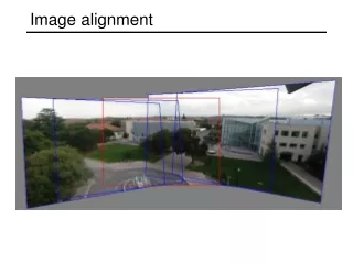
Image alignment • Goal: estimate single (u,v) translation for entire image • Easier subcase: solvable by pyramid-based Lukas-Kanade
Lucas-Kanade for image alignment • Pros: • All pixels get used in matching • Can get sub-pixel accuracy (important for good mosaicing!) • Relatively fast and simple • Cons: • Prone to local minima • Images need to be already well-aligned • What if, instead, we extract important “features” from the image and just align these?
Feature-based alignment • Find a few important features (aka Interest Points) • Match them across two images • Compute image transformation as per Project #3 • How do we choose good features? • They must prominent in both images • Easy to localize • Think how you did that by hand in Project #3 • Corners!
Feature Matching • How do we match the features between the images? • Need a way to describe a region around each feature • e.g. image patch around each feature • Use successful matches to estimate homography • Need to do something to get rid of outliers • Issues: • What if the image patches for several interest points look similar? • Make patch size bigger • What if the image patches for the same feature look different due to scale, rotation, etc. • Need an invariant descriptor
Invariant Feature Descriptors • Schmid & Mohr 1997, Lowe 1999, Baumberg 2000, Tuytelaars & Van Gool 2000, Mikolajczyk & Schmid 2001, Brown & Lowe 2002, Matas et. al. 2002, Schaffalitzky & Zisserman 2002