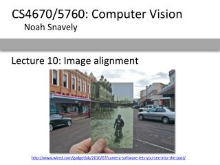
1. CS4670/5760: Computer Vision Noah Snavely Lecture 10: Image alignment http://www.wired.com/gadgetlab/2010/07/camera-software-lets-you-see-into-the-past/

2. Reading • Szeliski: Chapter 6.1

3. All 2D Linear Transformations • Linear transformations are combinations of … • Scale, • Rotation, • Shear, and • Mirror • Properties of linear transformations: • Origin maps to origin • Lines map to lines • Parallel lines remain parallel • Ratios are preserved • Closed under composition

4. Affine Transformations • Affine transformations are combinations of … • Linear transformations, and • Translations • Properties of affine transformations: • Origin does not necessarily map to origin • Lines map to lines • Parallel lines remain parallel • Ratios are preserved • Closed under composition

5. Projective Transformations aka Homographies aka Planar Perspective Maps Called a homography (or planar perspective map)

6. Homographies What happens when the denominator is 0?

7. Points at infinity

8. black area where no pixel maps to Image warping with homographies image plane in front image plane below

9. Homographies

10. 2D image transformations • These transformations are a nested set of groups • Closed under composition and inverse is a member

11. Questions?

12. Image Warping • Given a coordinate xform (x’,y’)= T(x,y) and a source image f(x,y), how do we compute an xformed image g(x’,y’)=f(T(x,y))? T(x,y) y’ y x x’ f(x,y) g(x’,y’)

13. Forward Warping • Send each pixel f(x) to its corresponding location (x’,y’)=T(x,y) in g(x’,y’) • What if pixel lands “between” two pixels? T(x,y) y’ y x x’ f(x,y) g(x’,y’)

14. Forward Warping • Send each pixel f(x,y) to its corresponding location x’=h(x,y) in g(x’,y’) • What if pixel lands “between” two pixels? • Answer: add “contribution” to several pixels, normalize later (splatting) • Can still result in holes T(x,y) y’ y x x’ f(x,y) g(x’,y’)

15. Inverse Warping • Get each pixel g(x’,y’) from its corresponding location (x,y)=T-1(x,y) in f(x,y) • Requires taking the inverse of the transform • What if pixel comes from “between” two pixels? T-1(x,y) y’ y x x’ f(x,y) g(x’,y’)

16. Inverse Warping • Get each pixel g(x’) from its corresponding location x’=h(x) in f(x) • What if pixel comes from “between” two pixels? • Answer: resample color value from interpolated (prefiltered) source image T-1(x,y) y’ y x x’ f(x,y) g(x’,y’)

17. Interpolation • Possible interpolation filters: • nearest neighbor • bilinear • bicubic (interpolating) • sinc • Needed to prevent “jaggies” and “texture crawl” (with prefiltering)

18. Computing transformations • Given a set of matches between images A and B • How can we compute the transform T from A to B? • Find transform T that best “agrees” with the matches

19. Computing transformations ?

20. Simple case: translations How do we solve for ?

21. Simple case: translations Displacement of match i = Mean displacement =

22. Another view • System of linear equations • What are the knowns? Unknowns? • How many unknowns? How many equations (per match)?

23. Another view • Problem: more equations than unknowns • “Overdetermined” system of equations • We will find the least squares solution

24. Least squares formulation • For each point • we define the residuals as

25. Least squares formulation • Goal: minimize sum of squared residuals • “Least squares” solution • For translations, is equal to mean displacement

26. Least squares formulation • Can also write as a matrix equation 2n x 2 2x 1 2n x 1

27. Least squares • Find t that minimizes • To solve, form the normal equations

28. Questions?