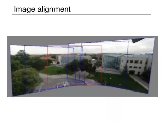
Image alignment
Image alignment. Image alignment: Motivation. Panorama stitching. Recognition of object instances. Image alignment: Challenges. Small degree of overlap. Occlusion, clutter. Image alignment. Two broad approaches: Direct (pixel-based) alignment Search for alignment where most pixels agree


Image alignment
E N D
Presentation Transcript
Image alignment: Motivation Panorama stitching Recognitionof objectinstances
Image alignment: Challenges Small degree of overlap Occlusion,clutter
Image alignment • Two broad approaches: • Direct (pixel-based) alignment • Search for alignment where most pixels agree • Feature-based alignment • Search for alignment where extracted features agree • Can be verified using pixel-based alignment
Alignment as fitting • Previous lectures: fitting a model to features in one image M Find model M that minimizes xi
xi xi ' T Alignment as fitting • Previous lectures: fitting a model to features in one image • Alignment: fitting a model to a transformation between pairs of features (matches) in two images M Find model M that minimizes xi Find transformation Tthat minimizes
Feature-based alignment outline • Extract features
Feature-based alignment outline • Extract features • Compute putative matches
Feature-based alignment outline • Extract features • Compute putative matches • Loop: • Hypothesize transformation T (small group of putative matches that are related by T)
Feature-based alignment outline • Extract features • Compute putative matches • Loop: • Hypothesize transformation T (small group of putative matches that are related by T) • Verify transformation (search for other matches consistent with T)
Feature-based alignment outline • Extract features • Compute putative matches • Loop: • Hypothesize transformation T (small group of putative matches that are related by T) • Verify transformation (search for other matches consistent with T)
2D transformation models • Similarity(translation, scale, rotation) • Affine • Projective(homography)
Let’s start with affine transformations • Simple fitting procedure (linear least squares) • Approximates viewpoint changes for roughly planar objects and roughly orthographic cameras • Can be used to initialize fitting for more complex models
Fitting an affine transformation • Assume we know the correspondences, how do we get the transformation?
Fitting an affine transformation • Linear system with six unknowns • Each match gives us two linearly independent equations: need at least three to solve for the transformation parameters
( ) ( ) What if we don’t know the correspondences? • Need to compare feature descriptors of local patches surrounding interest points ? ? = featuredescriptor featuredescriptor
Feature descriptors • Assuming the patches are already normalized (i.e., the local effect of the geometric transformation is factored out), how do we compute their similarity? • Want invariance to intensity changes, noise, perceptually insignificant changes of the pixel pattern
Feature descriptors • Simplest descriptor: vector of raw intensity values • How to compare two such vectors? • Sum of squared differences (SSD) • Not invariant to intensity change • Normalized correlation • Invariant to affine intensity change
p 2 0 Feature descriptors • Disadvantage of patches as descriptors: • Small shifts can affect matching score a lot • Solution: histograms
Feature descriptors: SIFT • Descriptor computation: • Divide patch into 4x4 sub-patches • Compute histogram of gradient orientations (8 reference angles) inside each sub-patch • Resulting descriptor: 4x4x8 = 128 dimensions David G. Lowe. "Distinctive image features from scale-invariant keypoints.”IJCV 60 (2), pp. 91-110, 2004.
Feature descriptors: SIFT • Descriptor computation: • Divide patch into 4x4 sub-patches • Compute histogram of gradient orientations (8 reference angles) inside each sub-patch • Resulting descriptor: 4x4x8 = 128 dimensions • Advantage over raw vectors of pixel values • Gradients less sensitive to illumination change • “Subdivide and disorder” strategy achieves robustness to small shifts, but still preserves some spatial information David G. Lowe. "Distinctive image features from scale-invariant keypoints.”IJCV 60 (2), pp. 91-110, 2004.
Feature matching • Generating putative matches: for each patch in one image, find a short list of patches in the other image that could match it based solely on appearance ?
Feature matching • Generating putative matches: for each patch in one image, find a short list of patches in the other image that could match it based solely on appearance • Exhaustive search • For each feature in one image, compute the distance to all features in the other image and find the “closest” ones (threshold or fixed number of top matches) • Fast approximate nearest neighbor search • Hierarchical spatial data structures (kd-trees, vocabulary trees) • Hashing
Feature space outlier rejection • How can we tell which putative matches are more reliable? • Heuristic: compare distance of nearest neighbor to that of second nearest neighbor • Ratio will be high for features that are not distinctive • Threshold of 0.8 provides good separation David G. Lowe. "Distinctive image features from scale-invariant keypoints.”IJCV 60 (2), pp. 91-110, 2004.
Reading David G. Lowe. "Distinctive image features from scale-invariant keypoints.”IJCV 60 (2), pp. 91-110, 2004.
Dealing with outliers • The set of putative matches contains a very high percentage of outliers • Heuristics for feature-space outlier rejection • Geometric fitting strategies: • RANSAC • Incremental alignment • Hough transform • Hashing
Strategy 1: RANSAC • RANSAC loop: • Randomly select a seed group of matches • Compute transformation from seed group • Find inliers to this transformation • If the number of inliers is sufficiently large, re-compute least-squares estimate of transformation on all of the inliers • Keep the transformation with the largest number of inliers
RANSAC example: Translation Putative matches
RANSAC example: Translation Select one match, count inliers
RANSAC example: Translation Select one match, count inliers
RANSAC example: Translation Select translation with the most inliers
Problem with RANSAC • In many practical situations, the percentage of outliers (incorrect putative matches) is often very high (90% or above) • Alternative strategy: restrict search space by using strong locality constraints on seed groups and inliers • Incremental alignment
Strategy 2: Incremental alignment • Take advantage of strong locality constraints: only pick close-by matches to start with, and gradually add more matches in the same neighborhood S. Lazebnik, C. Schmid and J. Ponce, “Semi-local affine parts for object recognition,”BMVC 2004.
Strategy 2: Incremental alignment • Take advantage of strong locality constraints: only pick close-by matches to start with, and gradually add more matches in the same neighborhood
Strategy 2: Incremental alignment • Take advantage of strong locality constraints: only pick close-by matches to start with, and gradually add more matches in the same neighborhood
Strategy 2: Incremental alignment • Take advantage of strong locality constraints: only pick close-by matches to start with, and gradually add more matches in the same neighborhood
Strategy 2: Incremental alignment • Take advantage of strong locality constraints: only pick close-by matches to start with, and gradually add more matches in the same neighborhood A
visual codeword withdisplacement vectors Strategy 3: Hough transform • Recall: Generalized Hough transform model test image B. Leibe, A. Leonardis, and B. Schiele, Combined Object Categorization and Segmentation with an Implicit Shape Model, ECCV Workshop on Statistical Learning in Computer Vision 2004
Strategy 3: Hough transform • Suppose our features are adapted to scale and rotation • Then a single feature match provides an alignment hypothesis (translation, scale, orientation) model David G. Lowe. "Distinctive image features from scale-invariant keypoints.”IJCV 60 (2), pp. 91-110, 2004.
Strategy 3: Hough transform • Suppose our features are adapted to scale and rotation • Then a single feature match provides an alignment hypothesis (translation, scale, orientation) • Of course, a hypothesis obtained from a single match is unreliable • Solution: let each match vote for its hypothesis in a Hough space with very coarse bins model David G. Lowe. "Distinctive image features from scale-invariant keypoints.”IJCV 60 (2), pp. 91-110, 2004.
Hough transform details (D. Lowe’s system) • Training phase: For each model feature, record 2D location, scale, and orientation of model (relative to normalized feature frame) • Test phase: Let each match between a test and a model feature vote in a 4D Hough space • Use broad bin sizes of 30 degrees for orientation, a factor of 2 for scale, and 0.25 times image size for location • Vote for two closest bins in each dimension • Find all bins with at least three votes and perform geometric verification • Estimate least squares affine transformation • Use stricter thresholds on transformation residual • Search for additional features that agree with the alignment David G. Lowe. "Distinctive image features from scale-invariant keypoints.”IJCV 60 (2), pp. 91-110, 2004.
Strategy 4: Hashing • Make each image feature into a low-dimensional “key” that indexes into a table of hypotheses hash table model
Strategy 4: Hashing • Make each image feature into a low-dimensional “key” that indexes into a table of hypotheses • Given a new test image, compute the hash keys for all features found in that image, access the table, and look for consistent hypotheses hash table test image model
Strategy 4: Hashing • Make each image feature into a low-dimensional “key” that indexes into a table of hypotheses • Given a new test image, compute the hash keys for all features found in that image, access the table, and look for consistent hypotheses • This can even work when we don’t have any feature descriptors: we can take n-tuples of neighboring features and compute invariant hash codes from their geometric configurations B C D A
Application: Searching the sky • http://www.astrometry.net/
Beyond affine transformations • Homography: plane projective transformation (transformation taking a quad to another arbitrary quad)
Homography • The transformation between two views of a planar surface • The transformation between images from two cameras that share the same center
Fitting a homography • Recall: homogenenous coordinates Converting from homogenenousimage coordinates Converting to homogenenousimage coordinates