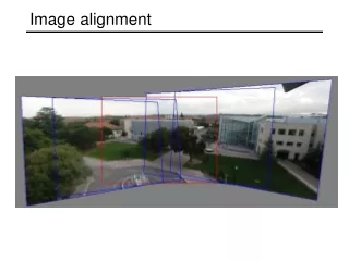
Image alignment
Image alignment. Image from http://graphics.cs.cmu.edu/courses/15-463/2010_fall/. A look into the past. http://blog.flickr.net/en/2010/01/27/a-look-into-the-past/. A look into the past. Leningrad during the blockade. http://komen-dant.livejournal.com/345684.html. Bing streetside images.
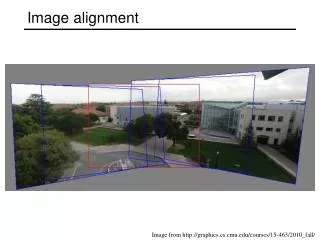

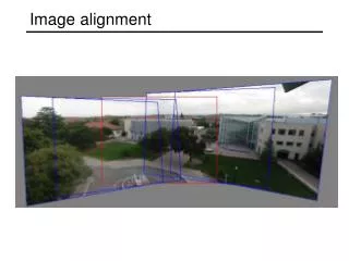
Image alignment
E N D
Presentation Transcript
Image alignment Image from http://graphics.cs.cmu.edu/courses/15-463/2010_fall/
A look into the past http://blog.flickr.net/en/2010/01/27/a-look-into-the-past/
A look into the past • Leningrad during the blockade http://komen-dant.livejournal.com/345684.html
Bing streetside images http://www.bing.com/community/blogs/maps/archive/2010/01/12/new-bing-maps-application-streetside-photos.aspx
Image alignment: Applications Panorama stitching Recognitionof objectinstances
Image alignment: Challenges Small degree of overlap Intensity changes Occlusion,clutter
Image alignment • Two families of approaches: • Direct (pixel-based) alignment • Search for alignment where most pixels agree • Feature-based alignment • Search for alignment where extracted features agree • Can be verified using pixel-based alignment
Alignment as fitting • Previous lectures: fitting a model to features in one image M Find model M that minimizes xi
xi xi ' T Alignment as fitting • Previous lectures: fitting a model to features in one image • Alignment: fitting a model to a transformation between pairs of features (matches) in two images M Find model M that minimizes xi Find transformation Tthat minimizes
2D transformation models • Similarity(translation, scale, rotation) • Affine • Projective(homography)
Let’s start with affine transformations • Simple fitting procedure (linear least squares) • Approximates viewpoint changes for roughly planar objects and roughly orthographic cameras • Can be used to initialize fitting for more complex models
Fitting an affine transformation • Assume we know the correspondences, how do we get the transformation?
Fitting an affine transformation • Linear system with six unknowns • Each match gives us two linearly independent equations: need at least three to solve for the transformation parameters
Fitting a plane projective transformation • Homography: plane projective transformation (transformation taking a quad to another arbitrary quad)
Homography • The transformation between two views of a planar surface • The transformation between images from two cameras that share the same center
Application: Panorama stitching Source: Hartley & Zisserman
Fitting a homography • Recall: homogeneous coordinates Converting fromhomogeneousimage coordinates Converting tohomogeneousimage coordinates
Fitting a homography • Recall: homogeneous coordinates • Equation for homography: Converting from homogeneousimage coordinates Converting to homogeneousimage coordinates
Fitting a homography • Equation for homography: 3 equations, only 2 linearly independent
Direct linear transform • H has 8 degrees of freedom (9 parameters, but scale is arbitrary) • One match gives us two linearly independent equations • Homogeneous least squares: find h minimizing ||Ah||2 • Eigenvector of ATA corresponding to smallest eigenvalue • Four matches needed for a minimal solution
Robust feature-based alignment • So far, we’ve assumed that we are given a set of “ground-truth” correspondences between the two images we want to align • What if we don’t know the correspondences?
Robust feature-based alignment • So far, we’ve assumed that we are given a set of “ground-truth” correspondences between the two images we want to align • What if we don’t know the correspondences? ?
Robust feature-based alignment • Extract features
Robust feature-based alignment • Extract features • Compute putative matches
Robust feature-based alignment • Extract features • Compute putative matches • Loop: • Hypothesize transformation T
Robust feature-based alignment • Extract features • Compute putative matches • Loop: • Hypothesize transformation T • Verify transformation (search for other matches consistent with T)
Robust feature-based alignment • Extract features • Compute putative matches • Loop: • Hypothesize transformation T • Verify transformation (search for other matches consistent with T)
( ) ( ) Generating putative correspondences • Need to compare feature descriptors of local patches surrounding interest points ? ? = featuredescriptor featuredescriptor
Feature descriptors • Recall: covariant detectors => invariant descriptors
Feature descriptors • Simplest descriptor: vector of raw intensity values • How to compare two such vectors? • Sum of squared differences (SSD) • Not invariant to intensity change • Normalized correlation • Invariant to affine intensity change
Disadvantage of intensity vectors as descriptors • Small deformations can affect the matching score a lot
Feature descriptors: SIFT • Descriptor computation: • Divide patch into 4x4 sub-patches • Compute histogram of gradient orientations (8 reference angles) inside each sub-patch • Resulting descriptor: 4x4x8 = 128 dimensions David G. Lowe. "Distinctive image features from scale-invariant keypoints.”IJCV 60 (2), pp. 91-110, 2004.
Feature descriptors: SIFT • Descriptor computation: • Divide patch into 4x4 sub-patches • Compute histogram of gradient orientations (8 reference angles) inside each sub-patch • Resulting descriptor: 4x4x8 = 128 dimensions • Advantage over raw vectors of pixel values • Gradients less sensitive to illumination change • Pooling of gradients over the sub-patches achieves robustness to small shifts, but still preserves some spatial information David G. Lowe. "Distinctive image features from scale-invariant keypoints.”IJCV 60 (2), pp. 91-110, 2004.
Feature matching • Generating putative matches: for each patch in one image, find a short list of patches in the other image that could match it based solely on appearance ?
Feature space outlier rejection • How can we tell which putative matches are more reliable? • Heuristic: compare distance of nearest neighbor to that of second nearest neighbor • Ratio of closest distance to second-closest distance will be highfor features that are not distinctive • Threshold of 0.8 provides good separation David G. Lowe. "Distinctive image features from scale-invariant keypoints.”IJCV 60 (2), pp. 91-110, 2004.
RANSAC • The set of putative matches contains a very high percentage of outliers • RANSAC loop: • Randomly select a seed group of matches • Compute transformation from seed group • Find inliers to this transformation • If the number of inliers is sufficiently large, re-compute least-squares estimate of transformation on all of the inliers • Keep the transformation with the largest number of inliers
RANSAC example: Translation Putative matches
RANSAC example: Translation Select one match, count inliers
RANSAC example: Translation Select one match, count inliers
RANSAC example: Translation Select translation with the most inliers
Scalability: Alignment to large databases • What if we need to align a test image with thousands or millions of images in a model database? • Efficient putative match generation • Approximate descriptor similarity search, inverted indices Test image ? Model database
Review: Alignment • Estimating transformation parameters • Affine • Projective (homography) • Robust alignment • Large-scale visual search
Large-scale visual search Reranking/ Geometric verification Inverted index Figure from: Kristen Grauman and Bastian Leibe, Visual Object Recognition, Synthesis Lectures on Artificial Intelligence and Machine Learning, April 2011, Vol. 5, No. 2, Pages 1-181
Large-scale visual search • What if we need to align a test image with thousands or millions of images in a model database? • Efficient putative match generation • Fast nearest neighbor search, inverted indexes Test image D. Nistér and H. Stewénius, Scalable Recognition with a Vocabulary Tree, CVPR 2006 Vocabulary tree with inverted index Database
Descriptor space Slide credit: D. Nister
Hierarchical partitioning of descriptor space (vocabulary tree) Slide credit: D. Nister
Vocabulary tree/inverted index Slide credit: D. Nister
Populating the vocabulary tree/inverted index Model images Slide credit: D. Nister