Download
1 / 75
810 likes | 1.14k Vues
AN OVERVIEW OF SIGMA-DELTA CONVERTERS. G. S. VISWESWARAN PROFESSOR ELECTRICAL ENGINEERING DEPARTMENT INDIAN INSTITUTE OF TECHNOLOGY, DELHI NEW DELHI 110 016 Email: gswaran@ee.iitd.ac.in Telephone: (011) 2659 1077; (011) 2685 2525. DOMAIN OF CONVERTERS. Sigma Delta. Successive Approx.

E N D
AN OVERVIEW OF SIGMA-DELTA CONVERTERS G. S. VISWESWARAN PROFESSOR ELECTRICAL ENGINEERING DEPARTMENT INDIAN INSTITUTE OF TECHNOLOGY, DELHI NEW DELHI 110 016 Email: gswaran@ee.iitd.ac.in Telephone: (011) 2659 1077; (011) 2685 2525
DOMAIN OF CONVERTERS Sigma Delta Successive Approx Subranging/Pipelined Flash Signal bandwidth converted
PCM NYQUIST RATE A/D CONVERTERS E[n] is a sample sequence of a random process uncorrelated with the sequence x[n]. The probability density of the error process is uniform over the range of quantization error i.e over /2 The error is a white noise process
PCM NYQUIST RATE A/D CONVERTERS The variance of the noise power for a quantization level is given by This gives us an SNR
PCM NYQUIST RATE A/D CONVERTERS In a Nyquist converter, the maximum signal to noise ratio that can be obtained for a sinusoidal input with a peak voltage of V is given by: Every additional bit 6dB of SNR. eg. Digital audio with signal bandwidth = 20kHz. If desired resolution = 18 bits SNR 110dB.
PCM NYQUIST RATE A/D CONVERTERS What is the problem with getting 18 bits of resolution ? 1. Nyquist rate converters essentially obtain output by comparing the input voltage to various reference levels. These reference levels are obtained by a process of reference division; using resistors or capacitors. Any mismatch in the resistors/capacitors results in loss of accuracy. 2. For an ‘N’ bit converter, the required matching of elements is at least 1 part in 2N. Matching of components to > 10 bits (or > 0.1 %) is difficult. 3. Nyquist rate converters require a sharp cutoff anti-aliasing filter.
OVERSAMPLED PCM CONVERTERS Oversampled converters attempt to use relatively imprecise analog components with additional digital signal processing circuits to achieve high resolution. This is done using Oversampling - the sampling frequency is much higher than the signal frequency
OVERSAMPLED PCM CONVERTERS Noise spectrum when sampled at fS >> 2fB Assume quantization noise is uniformly distributed, white and uncorrelated with the signal. Noise power folds back to –fS/2 to fS/2, oversampled converters have lower noise power within the signal band. Out of band noise can be removed by a digital filter following the PCM converter.
OVERSAMPLED PCM CONVERTERS We define Power Spectral Density of the output random Process is given by For an oversampled PCM converter |Hx(f)| = |He(f)| = 1. White noise assumption states that Pe(f) = Se2(f)/fs which implies Pey(f) = Sey2(f)/fs. Thus the in band noise power is given by
OVERSAMPLED PCM CONVERTERS We now see that the SNR ratio for this converter is The spectrum of the (over) sampled signal can represented as follows:
OVERSAMPLED PCM CONVERTERS “16-bit resolution digital audio” Oversampled 8-bit converter to be used. To get an SNR = 110dB with fB = 20kHz, we need fS 2.64GHz. This is still not good enough since the sampling frequency is too high. Further improvement can be obtained if noise shaping is used.
NOISE SHAPED OVERSAMPLED PCM CONVERTERS We see that for an A/D converter the output is given in general by Y(z) = X(z)Hx(z) + E(z)He(z) We have seen OS PCM converter using | Hx(z)| = | He(z)| = 1. We can however realize another converter using | Hx(z)| = 1 but choose He(z) to shape the noise spectrum to improve the noise performance. Noise shaping or modulation further attenuates noise in the signal band to other frequencies. The modulator output can be low pass filtered to attenuate the out of band noise and finally down sampled to get Nyquist rate samples.
NOISE SHAPED OVERSAMPLED PCM CONVERTERS Noise is high pass filtered to get additional resolution Simplest z- domain high pass filter: 1 –z-1We want an output Y(z) that contains the sun of the input and quantzation noise that is high pass filtered. i.e. Y(z) = X(z) + (1-z-1)E(z) or = z-1X(z) + (1- z-1)E(z)
NOISE SHAPED OVERSAMPLED PCM CONVERTERS Digital Analog One possibility is to first integrate the analog input, quantize it and then high pass filter it.
FIRST ORDER MODULATION The naïve system proposed has its own problems. The first problem is that since it is an open loop system, the integrator will saturate. It also requires matching between analog and digital portions of the circuit. Y(z) = z-1X(z) + (1 – z-1) E(z)
FIRST ORDER MODULATION Linearized ‘z’ domain model gives Hx(z) = STF = z-1 He(z) = NTF = 1-z-1 Assuming that the quantization noise is uncorrelated with the signal, Sxy(f) = Sx(f)Hx(f) 2 Sey(f) = Se(f)He(f) 2
FIRST ORDER MODULATION If fB<< fS Thus we obtain the Noise Power as
FIRST ORDER MODULATION Noise power coming out of First Order Modulator for an OSR of 128.
FIRST ORDER MODULATION Before we proceed to implement the transfer function we need to look in to certain realizatios in the sampled data domain. As the word implies there is an integration involved. In the continuous domain, this requires resistance and capacitance. As a designer we have the Capacity to Design but not the Resistance.
SWITCHED CAPACITOR CIRCUITS DOYEN OF SAMPLED DATA DESIGNS Sampled Signals: This gives a z transform
Realizing resistors for Sampled Data Circuits i1 i2 The average value of current i1 or i2 is given by This emulates a resistance of value R = T/C = 1/fC
SWITCHED CAP INTEGRATORS During 1 During 2 Using z transforms, this reduces to
SWITCHED CAP INTEGRATORS If << 1/T, and using z = exp(jT) we get H(ejT) as This circuit is then an integrator with a delay using the transformation s = (z-1)/T and is called the Forward Euler Integrator.
SWITCHED CAP INTEGRATORS This is another integrator that gives a non inverting integration at the output and uses the transformation s = (1-z-1)/T and is called the Backward Euler Integrator.
SWITCHED CAP INTEGRATORS The sampling capacitor Cs is now effectively Cs + CP, thus making the realized resistance R = T/(Cs + CP), different from the intended value --- needs correction, look for parasitic insensitive configuration.
SWITCHED CAP INTEGRATORS At 1 Cs gets charged to Vin(nT) and During 2 Giving us
SWITCHED CAP INTEGRATORS This configuration gives
BACK TO SIGMA DELTA CONVERTERS Implementation Imperfection in the first order sigma-delta modulator §Finite op-amp gain §Capacitance mismatch §Incomplete settling
FINITE OPAMP GAIN Using charge conservations at the nth clock cycle, we have: CSVI[n]- CSVd[n] = CF [Vo[n]+ Vd[n] – Vo[n-1] - Vd[n-1]] Using Vo[n] = Avd[n] and writing in z domain
FINITE OPAMP GAIN Output of the modulator is now given by where NTF denotes the noise transfer function and STF denotes the signal transfer function, NTF ‘0’ is shifted away from DC. Neglecting the effect of the pole in the NTF,
FINITE OPAMP GAIN = 1 +2-2 cos For small Noise power at the output is then
EFFECT OF FINITE BANDWIDTH Larger feedback factor lower gain faster setting Settling determines maximum clock frequency eg: CS = CF = 1pF = 0.5 Assume u = 100 MHz If we want setting to 1% error, time required 14.6ns clock frequency = 34MHz.
TIME DOMAIN BEHAVIOUR Y[n] = Y [n-1] + (X[n-1] – V[n-1]) if Y[n] 0 Y[n] = 1.0 else Y[n] = - 1.0
Y[n] V[n] 0 0.0 1 0.33 1 2 -0.33 -1 3 1 1 4 0.33 1 5 -0.33 -1 6 1 1 TIME DOMAIN BEHAVIOUR For example, for a DC input = , the time domain output for the first six clock cycles is given by: It can be seen that the average value of the output is 1/3
TIME DOMAIN BEHAVIOUR (Non Linear) §Quantization error spectrum is not white; successive output levels may be correlated. §Limit cycle oscillations that lead to tones in the output eg. DC input X[n] = x For a limit cycle of period T; V[n] = V[n+T] Y[n] = Y[n+T] Since the input is DC, the input to the integrator will also be periodic.
TIME DOMAIN BEHAVIOUR (Non Linear) Now Y[n] – Y[n-1] = X – V[n-1]. Write this equation for ‘T’ time instances and add; we get but Y[T] = Y [0]
PATTERN NOISE IN MODULATOR It should be clear that the MODULATOR is expected to give out the output equal to the DC input. Only limited no. of levels are allowed to the output , therefore output has to toggle from one level to another in order to keep average output equal to the DC input. For eg. Input=0.5 Levels allowed are 0 and 1 Then the output will toggle between 0 and 1. If average is taken then the value of output of SDM is 0.5. Therefore the output is oscillating with a frequency half of that of fs. That means in frequency domain the output will have tones at fs/2 and fs.
PATTERN NOISE IN MODULATOR Similarly for dc level of 1/256, the output will have, one one and 255 zeroes in 256 clocks (fs) this means the output will oscillate at a frequency of (fs/256). Hence it will have tones lying at multiples of this frequency. As the dc level comes closer to zero the tonal frequency decreases. The tones are completely harmless till they are out of the signal bandwidth. The thing to note over here is that these tones represent noise as the information or signal is at 0 frequency rest of the frequency components are noise. This effect is very much prominent in I order modulators. Another important fact is that the amplitudes of the tones decrease as they come closer to the signal bandwidth. It is always better to analyze them by using simulations.
PATTERN NOISE IN MODULATOR The question to be asked is why are this tones dangerous in the signal bandwidth? The answer to this question lies in the fact that all the analysis made earlier on was based on the white noise approximation and the problem with the tones is that they are much above the expected noise floor. Hence the true signal to noise ratio is much lesser than what was expected from the analysis.