Understanding Hidden Markov Models in Spoken Language Processing
In this lecture by Prof. Andrew Rosenberg, the concepts of the Hidden Markov Model (HMM) in speech processing are explored. The Markov assumption is discussed, emphasizing that future states depend only on the present state, not the past. The lecture covers the Forward-Backward Algorithm for training HMMs, detailing how observations are used to update state probabilities. Additionally, Viterbi Decoding is introduced for finding the most likely state sequences given observations. Applications in acoustic modeling and forced alignment are also examined.

Understanding Hidden Markov Models in Spoken Language Processing
E N D
Presentation Transcript
Sequential Modeling with the Hidden Markov Model Lecture 9 Spoken Language Processing Prof. Andrew Rosenberg
Markov Assumption • If we can represent all of the information available in the present state, encoding the past is un-necessary. The future is independent of the past given the present
Markov Assumption in Speech • Word Sequences • Phone Sequences • Part of Speech Tags • Syntactic constituents • Phrase sequences • Discourse Acts • Intonation
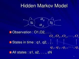
Markov Chain • The probability of a sequence can be decomposed into a probability of sequential events. x1 x2 x3
Hidden Markov model • In a Hidden Markov Model the state sequence is unobserved. • Only an observation sequence is available q1 q2 q3 x1 x2 x3
Hidden Markov model • Observations are MFCC vectors • States are phone labels • Each state (phone) has an associated GMM modeling the MFCC likelihood q1 q2 q3 x1 x2 x3
Forward-Backwards Algorithm • HMMs are trained by collecting and distributing information from observations to states. • The Forward-Backwards algorithm is a specific example of EM. • In the HMM topology (variable relationship), the training converges in one forward pass, and a backwards pass. • hence the name
Forwards Backwards Algorithm • Forwards-Step: • Collect up from the observations to the states • Collect from left state to right state. • “Collect” – update parameters to correctly model the observations • Observation collection will give a distribution over states, given the initial state • State collection will also give a distribution over states • the new q distribution will reflect the combination of these two q1 q2 q3 x1 x2 x3
Forwards Backwards Algorithm • Backwards-Step: • Distribute down to the observations from the states • Collect from left state to right state. • “Distribute” – update parameters to correctly model the observations • Observation distribute updates the state-observation relationship • State distribution updates the state-state transition matrix • Forward-backwards can be shown to converge in one pass. q1 q2 q3 x1 x2 x3
Finite State Automata • “Start” “Accept” States • Epsilon Transitions • Relationship to Regular Expressions • Operations on FSA • Addition • Inversion • Node expansion • Determinization • Weighted automata allow probabilities to be assigned to transitions
State transitions as FSA /d/ /t/ /ey/ /ax/ /ae/ /dx/
Word FSA to phone FSA MORE DATA /d/ /t/ /ey/ /ax/ /ae/ /dx/ /m/ /ao/ /r/
Word FSA to phone FSA /d/ /t/ /ey/ /ax/ /ae/ /dx/ /m/ /ao/ /r/
Decoding a Hidden Markov Model • Decoding is finding the most likely state sequence. • How many state sequences are there in a HMM with N observations and k states?
Viterbi Decoding • Dynamic Programming can make this a lot faster. • Idea: Any optimal sequence between x0 and xnmust include the optimal sequence between xn and xn-1. • Based on the Markov Assumption.
Viterbi Decoding • Probability of most likely state sequence • Recovering the the optimal sequence involves storing pointers as decisions are made.
Example (from Wikipedia) states = ('Rainy', 'Sunny') observations = ('walk', 'shop', 'clean') start_probability = {'Rainy': 0.6, 'Sunny': 0.4} transition_probability = { 'Rainy' : {'Rainy': 0.7, 'Sunny': 0.3}, 'Sunny' : {'Rainy': 0.4, 'Sunny': 0.6}, } emission_probability = { 'Rainy' : {'walk': 0.1, 'shop': 0.4, 'clean': 0.5}, 'Sunny' : {'walk': 0.6, 'shop': 0.3, 'clean': 0.1}, } What is the most likely state sequence?
HMM Topology for Training • Rather than having one GMM per phone, it is common for acoustic models to represent each phone as 3 triphones S3 S2 S4 /r/ S5 S1
Flat Start • In Flat Start training, GMM parameters are initialized to global means and variances. • Viterbi is used to perform forced alignmentbetween observations and phone sequence. • The phone sequence is derived from the lexical transcription and pronunciation model
Forced Alignment • Given a phone sequence and observations, assign each observation to a phone. • Uses • Identifying which observation belong to each phone label for later training • Getting time boundaries for phone or word labels.
Flat Start • In Flat Start training, GMM parameters are initialized to global means and variances. • Viterbi is used to perform forced alignmentbetween observations and phone sequence. • The phone sequence is derived from the lexical transcription and pronunciation model • After alignment, retrain Acoustic Models, and repeat.
What about silence? • If there is no “silence” state, the silent frames will be assigned to either the /d/ or the /ax/ • This leads to worse acoustic models. • A solution: Explicit training of silence models, /sp/ • Allowing /sp/ transitions at word boundaries /d/ /ey/ /dx/ /ax/ /d/ /ey/ /dx/ /ax/ /d/ /ey/ /dx/ /ax/
Next Class • Pronunciation Modeling • Reading: J&M Chapter 2, Section10.5.3, 11.1, 11.2