Understanding Conditional Probability and Independence in Events
Learn the basics of conditional probability, how to calculate it, and understand the concept of independent events in probability theory. Explore practical examples and rules to grasp these fundamental concepts.

Understanding Conditional Probability and Independence in Events
E N D
Presentation Transcript
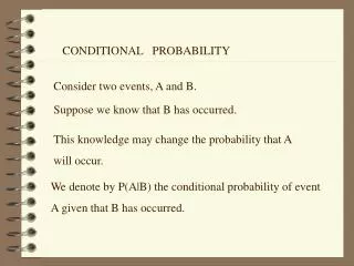
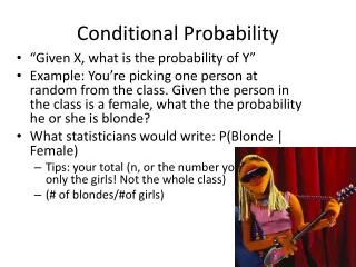
Conditional Probability As we have seen, P(A) refers to the probability that event A will occur. P(A|B) refers to the probability that A will occur but with the understanding that B has already occurred and we know it. So, we say the probability of A given B. The given B part means that it is known that B has occurred. By definition P(A|B) = P(A and B)/P(B). Similarly P(B|A) = P(A and B)/P(A). Note P(A and B) = P(B and A)
Now we have by definition P(A|B) = P(A and B)/P(B). In this definition, B has already occurred. The P(B) is the denominator of P(A|B) and is thus the base of the conditional probability. The intersection of A and B is in the numerator. Since B has occurred, the only way A can have occurred is if there is an overlap of A and B. So we have the ratio probability of overlap/probability of known event. Let’s turn to our example from the previous section
Conditional probability from joint probability table Actually Purchased Planned to purchase B (Yes) B’ (No) Total A (Yes) 0.20 0.05 0.25 A’ (No) 0.10 0.65 0.75 Total 0.30 0.70 1.0 So, if we know B has occurred then we look at column B. The only way A could also have occurred is if we had the joint event A and B. Thus, P(A|B) = .2/.3 = .67 Similarily, if we know A has occurred then we look at the row A. The only way B could also have occurred is if we had the joint event A and B. P(B|A) = .2/.25 = .8
In the example on the last slide P(A) = .25, but P(A|B) = .67. Each is dealing with the probability of A. But, in this case having information about B gives a different view about A. When P(A|B) ≠ P(A) we say events A and B are dependent events. Similarly, when P(B|A) ≠ P(B) events A and B are dependent. In our example, .25 of the folks in general have what we called event A (planned to purchase). But, the conditional probability is indicating that if we know B occurred (a purchase was actually made) then the chance is even higher (in this case) that they planned to purchase. In this sense A and B are dependent. Independent Events Events A and B are said to be independent if P(A|B) = P(A) or P(B|A) = P(B).
Does a coin have a memory? In other words, does a coin remember how many times it has come up heads and will thus come up tails if it came up heads a lot lately? Say A is heads on the third flip, B is heads on the first two flips. Is heads on the third flip influenced by the first two heads. No, coins have no memory! Thus A and B are independent. (Note I am not concerned here about the probability of getting three heads!) Have you ever heard the saying, “Pink sky in the morning, sailors take warning, pink sky at night sailors delight.” I just heard about it recently. Apparently it is a rule of thumb about rain. Pink sky in the morning would serve as a warning for rain that day. If A is rain in the day and B is pink sky in the morning, then it seems that the P(A|B) ≠ P(A) and thus the probability of rain is influenced by morning sky color (color is really just an indicator of conditions).
I have used these two examples to give you a feel about when events are independent and when they are dependent. By simple equation manipulation we change the conditional probability definition to the rule called the multiplication lawor rule for the intersection of events: P(A and B) = P(B)P(A⃒B) or P(A and B) = P(A)P(B⃒A) . Note the given part shows up in the other term. Now this rule simplifies if A and B are independent. The conditional probabilities revert to regular probabilities. We would then have P(A and B) = P(B)P(A) = P(A)P(B).
Say, as a new example, we have A and B with P(A)=.5, P(B)=.6 and P(A and B) =.4 Then a. P(A⃒B) = .4/.6 = .667 b. P(B⃒A) = .4/.5 = .8 c. A and B are not independent because we do NOT have P(A⃒B) = P(A), or P(B⃒A) = P(B). Say, as another example, we have A and B with P(A)=.3 and P(B)=.4 and here we will say A and B are mutually exclusive. This means P(A and B) = 0 (in a Venn Diagram A and B have no overlap), then a. P(A⃒B) = 0/.4 = 0 Here A and B are not independent.
Y Y1 Y2 Totals X X1 P(X1 andY1) P(X1 andY2) P(X1) X2 P(X2 andY1) P(X2 andY2) P(X2) Totals P(Y1) P(Y2) 1.00 Here I put the joint probability table again in general terms. Question X has mutually exclusive and collectively exhaustive events X1 and X2. For Y we have a similar set-up. Note here each has only two responses, but what we will see below would apply if there are more than 2 responses. Let’s review some of the probability rules we just went through and then we will add one more rule.
Inside the joint probability table we find joint probabilities (like P(X1 and Y1) and in the margins we find the marginal probabilities (like P(X1)). Marginal Probability Rule P(X1) = P(X1 and Y1) + P(X1 and Y2) General Addition Rule P(X1 or Y1) = P(X1) + P(Y1) – P(X1 and Y1) Conditional Probability P(X1|Y1) = P(X1 and Y1)/P(Y1) Multiplication Rule P(X1 and Y1) = P(X1|Y1)P(Y1)
The new part is to view the marginal probability rule as taking each part and use the multiplication rule. So, Marginal Probability Rule P(X1) = P(X1 and Y1) + P(X1 and Y2) =P(X1|Y1)P(Y1) + P(X1|Y2)P(Y2) Where Y1 and Y2 are mutually exclusive and collectively exhaustive.
example The joint probability table associated with the problem is B B’ total A .11 .22 .33 A’ .22 .44 .66 total .33 .67 1.0 (Some off due to rounding) P(A|B) = .11/.33 = .33, P(A|B’) = .22/.67 = .33 P(A’|B) = .22/.33 = .67 Since P(A) = P(A|B) = .33 events A and B are independent. To see if you have independent events you just compare the marginal (like P(A)) with the conditional (like P(A|B)). If equal, you have independent events.
Problem 4.22 page 138 The joint probability table associated with the problem is (no particles)B B’ total Good A .71 .03 .74 Bad A’ .18 .08 .26 total .89 .11 1.0 a. P(B’|A’) = .08/.26 = .31, b. P(B’|A) = .03/.74 = .04 c. P(B|A) = .71/.74 = .96. Since P(B) = .89 ≠ P(B|A) the events A and B are NOT independent. To see if you have independent events you just compare the marginal (like P(B)) with the conditional (like P(B|A)). If equal, you have independent events.