Understanding Exponential, Logarithmic, and Logistic Growth Models in Statistics
Explore the fundamental concepts of exponential growth, decay, and logistic growth models. Discover how the Gaussian model, also known as the bell curve, applies to real-valued random variables and their clustering around a mean. The exponential equations illustrate growth and decay dynamics, while the logistic model captures population growth in an S-shaped curve, demonstrating initial rapid growth followed by saturation. Learn about the equations and applications of these models in real-world scenarios, including population dynamics and statistical analysis.

Understanding Exponential, Logarithmic, and Logistic Growth Models in Statistics
E N D
Presentation Transcript
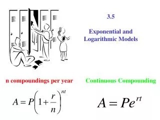
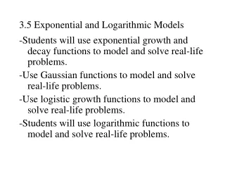
3.5 Exponential and Logarithmic Models Gaussian Model Logistic Growth model Exponential Growth and Decay
Gaussian Model or the Bell curve The normal (or Gaussian) distribution is a continuous probability distribution that is often used as a first approximation to describe real-valued random variables that tend to cluster around a single mean value. The graph of the associated probability density function is "bell"-shaped, and is known as the Gaussian function or bell curve:
Gaussian Model or the Bell curve If I was curving your grades, 68.2% of the students would have a C, 13.6% a B or D and 2.1% a A or F. 0.1% would have an A+
Gaussian Model or the Bell curve Its equations would be y = ae-[(x –b)^2]/c , where a ,b and c are real numbers.
y = ae-[(x –b)^2]/c Let a = 4; b = 2 and c = 3. The graph will never touch the x axis.
Exponential Growth/ Decay models Growth equation y = aebx b> 0 Decay equation y = ae-bx b>0 Both these models we have seen before in Algebra 2 and in Pre- Cal
Growth equation y = aebx Let a = 5 and b = 2
Decay equation y = ae-bx Let a = 2 and b = 2
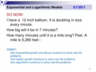
Will a small lake have exponential growth of game fish forever? No, What are the factors that keep the lake from the lake filling up with fish?
Logistic growth model • A logistic function or logistic curve is a common sigmoid curve, given its name in 1844 or 1845 by Pierre François Verhulst who studied it in relation to population growth. It can model the "S-shaped" curve (abbreviated S-curve) of growth of some population P. The initial stage of growth is approximately exponential; then, as saturation begins, the growth slows, and at maturity, growth stops. Pierre Francois Verhuist http://en.wikipedia.org/wiki/Logistic_function
Logistic Growth Model a, b and r are positive numbers. a is the maximum limit of the function.
Logistic Growth Model Let a = 10, b = 4 and r = 2
Homework Page 243- 248 # 18, 25, 28, 29, 35, 40 , 47, 50, 63, 70, 74, 93