Power Network Distribution
Power Network Distribution. Chung-Kuan Cheng CSE Dept. University of California, San Diego. Research Projects. SPICE_Diego Whole chip simulation using cloud computing Power Distribution: Analysis, Synthesis, Methodology 3D IC pathfinder Interconnect: Analysis, Synthesis

Power Network Distribution
E N D
Presentation Transcript
Power Network Distribution Chung-Kuan Cheng CSE Dept. University of California, San Diego
Research Projects • SPICE_Diego • Whole chip simulation using cloud computing • Power Distribution: Analysis, Synthesis, Methodology • 3D IC pathfinder • Interconnect: Analysis, Synthesis • Eye diagram prediction under power ground noises • Physical Layout • Performance driven placement
Research on Power Distribution Networks • Analysis • Stimulus, Noise Margin, Simulation • Synthesis • VRM, Decap, ESR, Topology • Integration • Sensors, Prediction, Stability, Robustness
Power Distribution Network Overview • Background: power distribution networks (PDN’s) • Analysis: worst-case PDN noise prediction • Target Impedance • Worst Current Loads • Rogue Wave • Conclusions and future work
Introduction: Motivation ITRS Roadmap: MPU SoC
What is a power distribution network (PDN) • Power supply noise • Resistive IR drop • Inductive Ldi/dt noise [Popovich et al. 2008]
Resonant Phenomenon: One-Stage LC Tank w/ ESR’s Y(jw) at current load: • If we ignore R1 and R2 Y(jw)=jwC+1/jwL=j(wC-1/wL) • When w= (CL)-1/2, we have Y(jw) --> 0. Impedance at load: Z(jw)= 1/Y(jw) --> inf
Introduction • Target Impedance = Vdd/Iload x 5% • Production Cost • Negative Noise Budget • Negotiation between IC and package • Activity scheduling
Analysis: Motivation • Target Impedance • Impedance in frequency domain • Worst power load in time domain • Slope of power load stimulus • Composite effect of resonance at multiple frequencies
Target Impedance • PDN design • Objective: low power supply noise • Popular methodology: “target impedance” [Smith ’99] • Implication: if the target impedance is small, then the noise will also be small
Analysis: Formulation • Problems with “target impedance” design methodology • How to set the target impedance? • Small target impedance may not lead to small noise • A PDN with smaller Zmax may have larger noise • Time-domain design methodology: worst-case PDN noise • If the worst-case noise is smaller than the requirement, then the PDN design is safe. • Straightforward and guaranteed • How to generate the worst-case PDN noise FT: Fourier transform
Analysis: Related Work • At final design stages [Evmorfopoulos ’06] • Circuit design is fully or almost complete • Realistic current waveforms can be obtained by simulation • Problem: countless input patterns lead to countless current waveforms • Sample the excitation space • Statistically project the sample’s own worst-case excitations to their expected position in the excitation space • At early design stages [Najm ’03 ’05 ’07 ’08 ’09] • Real current information is not available • “Current constraint” concept • Vectorless approach: no simulation needed • Problem: assume ideal current with zero transition time
Analysis: Formulation • Problem formulation I • PDN noise: • Worst-case current [Xiang ’09]: Zero current transition time. Unrealistic!
Ideal Case Study: One-Stage LC Tank w/ ESR’s • Define: • Note • Under-damped condition:
Ideal Case Study: One-Stage LC Tank w/ ESR’s (Cont’) • Step response: where • Normalized step response:
Ideal Case Study: One-Stage LC Tank w/ ESR’s (Cont’) • Local extreme points of the step response: • Normalized magnitude of the first peak:
Ideal Case Study: One-Stage LC Tank w/ ESR’s (Cont’) • Normalized worst-case noise:
Ideal Case Study: One-Stage LC Tank w/ ESR’s (Cont’) • Impedance: • When [Mikhail 08] • Normalized peak impedance:
Analysis: Algorithms • Problem formulation II T: chosen to be such that h(t) has died down to some negligible value. * f(t) replaces i(T-τ)
Proposed Algorithm Based on Dynamic Programming • GetTransPos(j,k1,k2):find the smallest i such that Fj(k1,i)≤ Fj(k2,i) • Q.GetMin(): return the minimum element in the priority queue Q • Q.DeleteMin(): delete the minimum element in the priority queueQ • Q.Add(e): insert the element e in the priority queueQ
Proposed Algorithm: Initial Setup • Divide the time range [0, T]into m intervals [t0=0, t1], [t1, t2], …, [tm-1, tm=T]. h(ti) = 0, i=1, 2, …, m-1 • u0 = 0, u1, u2, …, un = b are a set of n+1 values within [0, b].The value of f(t) is chosen from those values. A larger n gives more accurate results. h(t)
Proposed Algorithm: f(t) within a time interval [tj, tj+1] h(t) Theorem 1: The worst-case f(t) can be cons-tructed by determining the values at the zero-crossing points of the h(t) • Ij(k,i): worst-case f(t) starting with uk at time tj and ending with ui at time tj+1
Proposed Algorithm: Dynamic Programming Approach • Define Vj(k,i): the corresponding output within time interval [tj, tj+1] • Define the intermediate objective function OPT(j,i): the maximum output generated by the f(t) ending at time tj with the value ui • Recursive formula for the dynamic programming algorithm: • Time complexity:
Acceleration of the Dynamic Programming Algorithm • Without loss of generality, consider the time interval [tj, tj+1] where h(t) is negative. • Define Wj(k,i): the absolute value of Vj(k,i): Lemma 1: Wj(k2,i2)- Wj(k1,i2)≤ Wj(k2,i1)- Wj(k1,i1) for any 0 ≤ k1 < k2 ≤ n and 0 ≤ i1 < i2 ≤ n
Acceleration of the Dynamic Programming Algorithm • Define Fj(k,i): the candidate corresponding to k for OPT(j,i) • Accelerated algorithm: • Based on Theorem 2 • Using binary search and priority queue Theorem 2: Suppose k1 < k2, i1∈[0,n]and Fj(k1,i1)≤ Fj(k2,i1), then for any i2 > i1, we have Fj(k1,i2)≤ Fj(k2,i2).
Analysis: Case Study • Case 1: Impedance => Voltage drop • Transition Time • Case 2: Impedances vs. Worst Cases • Case 3: Voltage drop due to resonance at multiple frequencies.
Case Study 1: Impedance 3.23mΩ @ 166MHz 2.09mΩ @ 19.8KHz 1.69mΩ @ 465KHz
Case Study 1: Impulse Response Impulse response: 0s~100ns High frequency oscillation at the beginning with large amplitude, but dies down very quickly Amplitude = 1861 Low frequency oscillation with the smallest amplitude, but lasts the longest Mid-frequency oscillation with relatively small amplitude. Impulse response: 10µs~100µs Impulse response: 100ns~10µs Amplitude = 0.01 Amplitude = 29
Case Study 1: Worst-Case Current • Current constraints: Zoom in • The worst-case current also oscillates with the three resonant frequencies which matches the impulse response. • Saw-tooth-like current waveform at large transition times
Case Study 1: Worst-Case Noise vs.. Transition Time • The worst-case noise decreases with transition times. • Previous approaches which assume zero current transition times result in pessimistic worst-case noise.
Case Study 2: Impedances vs. Worst Cases 101.6MHz 98.1MHz 10.9MHz 224.3KHz 224.3KHz 11.2MHz
Case Study 2: Worst-Case Noise • for both cases: meaning that the worst-case noise is larger than Zmax. • The worst-case noise can be larger even though its peak impedance is smaller.
Case 3: “Rogue Wave” Phenomenon • Worst-case noise response: The maximum noise is formed when a long and slow oscillation followed by a short and fast oscillation. • Rogue wave: In oceanography, a large wave is formed when a long and slow wave hits a sudden quick wave. High-frequency oscillation corresponds to the resonance of the 1st stage Low-frequency oscillation corresponds to the resonance of the 2nd stage
Case 3: “Rogue Wave” Phenomenon (Cont’) Equivalent input impedance of the 2nd stage at high frequency
Case 3: “Rogue Wave” Phenomenon (Cont’) • Input current i(t): • Blue (I1): worst-case input stimulus • Red (I2): low frequency part of I1 • Green (I3): high frequency part of I1 I1=I2+I3
Case 3: “Rogue Wave” Phenomenon (Cont’) • Input current i(t) (zoom in):
Case 3: “Rogue Wave” Phenomenon (Cont’) • Noise response @ chip output • Blue (V1): response of I1 • Red (V2): response of I2 • Green (V3): response of I3
Case 3: “Rogue Wave” Phenomenon (Cont’) • Noise response (zoom in):
Remarks • Worst-case PDN noise prediction with non-zero current transition time • Current model is crucial for analysis • The worst-case PDN noise decreases with transition time • Small peak impedance may not lead to small worst-case noise • “Rogue wave” phenomenon • Adaptive parallel flow for PDN simulation using DFT • 0.093% relative error compared to SPICE • 10x speed up with single processor. • Parallel processing reduces the simulation time even more significantly
Summary • Power Distribution Network • VRMs, Switches, Decaps, ESRs, Topology, • Analysis • Stimulus, Noise Tolerance, Simulation • Control (smart grid) • High efficiency, Real time analysis, Stability, Reliability, Rapid recovery, and Self healing
Publication List • Power Distribution Network Simulation and Analysis [1] W. Zhang and C.K. Cheng, "Incremental Power Impedance Optimization Using Vector Fitting Modeling,“ IEEE Int. Symp. on Circuits and Systems, pp. 2439-2442, 2007. • [2] W. Zhang, W. Yu, L. Zhang, R. Shi, H. Peng, Z. Zhu, L. Chua-Eoan, R. Murgai, T. Shibuya, N. Ito, and C.K. Cheng, "Efficient Power Network Analysis Considering Multi-Domain Clock Gating,“ IEEE Trans on CAD, pp. 1348-1358, Sept. 2009. [3] W.P. Zhang, L. Zhang, R. Shi, H. Peng, Z. Zhu, L. Chua-Eoan, R. Murgai, T. Shibuya, N. Ito, and C.K. Cheng, "Fast Power Network Analysis with Multiple Clock Domains,“ IEEE Int. Conf. on Computer Design, pp. 456-463, 2007. [4] W.P. Zhang, Y. Zhu, W. Yu, R. Shi, H. Peng, L. Chua-Eoan, R. Murgai, T. Shibuya, N. Ito, and C.K. Cheng, "Finding the Worst Case of Voltage Violation in Multi-Domain Clock Gated Power Network with an Optimization Method“ IEEE DATE, pp. 540-547, 2008. [5] X. Hu, W. Zhao, P. Du, A.Shayan, C.K.Cheng, “An Adaptive Parallel Flow for Power Distribution Network Simulation Using Discrete Fourier Transform,” IEEE/ACM Asia and South Pacific Design Automation Conference (ASP-DAC), 2010. [6] C.K. Cheng, P. Du, A.B. Kahng, G.K.H. Pang, Y. Wang, and N. Wong, "More Realistic Power Grid Verification Based on Hierarchical Current and Power Constraints,“ ACM Int. Symp. on Physical Design, pp. 159-166, 2011.
Publication List • Power Distribution Network Analysis and Synthesis • [7] W. Zhang, Y. Zhu, W. Yu, A. Shayan, R. Wang, Z. Zhu, C.K. Cheng, "Noise Minimization During Power-Up Stage for a Multi-Domain Power Network,“ IEEE Asia and South Pacific Design Automation Conf., pp. 391-396, 2009. • [8] W. Zhang, L. Zhang, A. Shayan, W. Yu, X. Hu, Z. Zhu, E. Engin, and C.K. Cheng, "On-Chip Power Network Optimization with Decoupling Capacitors and Controlled-ESRs,“Asia and South Pacific Design Automation Conference, 2010. [9] X. Hu, W. Zhao, Y.Zhang, A.Shayan, C. Pan, A. E.Engin, and C.K. Cheng, “On the Bound of Time-Domain Power Supply Noise Based on Frequency-Domain Target Impedance,” System Level Interconnect Prediction Workshop (SLIP), July 2009. [10] A. Shayan, X. Hu, H. Peng, W. Zhang, and C.K. Cheng, “Parallel Flow to Analyze the Impact of the Voltage Regulator Model in Nanoscale Power Distribution Network,” In. Symp. on Quality Electronic Design (ISQED), Mar. 2009. [11] X. Hu, P. Du, and C.K. Cheng, "Exploring the Rogue Wave Phenomenon in 3D Power Distribution Networks,“ IEEE Electrical Performance of Electronic Packaging and Systems, pp. 57-60, 2010. • [12] C.K. Cheng, A.B. Kahng, K. Samadi, and A. Shayan, "Worst-Case Performance Prediction Under Supply Voltage and Temperature Variation,“ ACM/IEEE Int. Workshop on System Level Interconnect Prediction, pp. 91-96, 2010.
Publication List (Cont’) • 3D Power Distribution Networks • [13] A. Shayan, X. Hu, “Power Distribution Design for 3D Integration”, Jacob School of Engineering Research Expo, 2009 [Best Poster Award] • [14] A. Shayan, X. Hu, M.l Popovich, A.E. Engin, C.K. Cheng, “Reliable 3D Stacked Power Distribution Considering Substrate Coupling”, in International Conference on Computer Design (ICCD), 2009. [15] A. Shayan, X. Hu, C.K. Cheng, “Reliability Aware Through Silicon Via Planning for Nanoscale 3D Stacked ICs,” in Design, Automation & Test in Europe Conference (DATE), 2009. [16] A. Shayan, X. Hu, H. Peng, W. Zhang, C.K. Cheng, M. Popovich, and X. Chen, “3D Power Distribution Network Co-design for Nanoscale Stacked Silicon IC,” in 17th Conference on Electrical Performance of Electronic Packaging (EPEP), Oct. 2008. [5] [17] W. Zhang, W. Yu, X. Hu, A. Shayan, E. Engin, C.K. Cheng, "Predicting the Worst-Case Voltage Violation in a 3D Power Network", Proceeding of IEEE/ACM International Workshop on System Level Interconnect Prediction (SLIP), 2009. [18] X. Hu, P. Du, and C.K. Cheng, "Exploring the Rogue Wave Phenomenon in 3D Power Distribution Networks,“ IEEE Electrical Performance of Electronic Packaging and Systems, pp. 57-60, 2010.