Download
1 / 61
610 likes | 636 Vues
This presentation discusses the history and motivation behind Support Vector Machines (SVMs), as well as the use of margin-based loss for classification and regression problems. It explores the optimization formulation and the convex hull interpretation of the dual form of SVMs.

E N D
Part 2:Margin-Based Methods and Support Vector Machines Vladimir Cherkassky University of Minnesota cherk001@umn.edu Presented at Chicago Chapter ASA, May 6, 2016 Electrical and Computer Engineering 1 1
SVM: Brief History Margin (Vapnik & Lerner) Margin(Vapnik and Chervonenkis, 1964) 1964 RBF Kernels (Aizerman) 1965 Optimization formulation (Mangasarian) 1971 Kernels (Kimeldorf annd Wahba) 1992-1994 SVMs (Vapnik et al) 2000 – present Rapid growth, numerous apps Extensions to other problems
MOTIVATION for SVM Recall ‘conventional’ methods: - model complexity ~ dimensionality (# features) - nonlinear methods multiple minima - hard to control complexity ‘Good’ learning method: (a) tractable optimization formulation (b) tractable complexity control(1-2 parameters) (c) flexible nonlinear parameterization Properties (a), (b) hold for linear methods SVM solution approach
SVM APPROACH Linear approximation in Z-space using special adaptive loss function Complexity independent of dimensionality
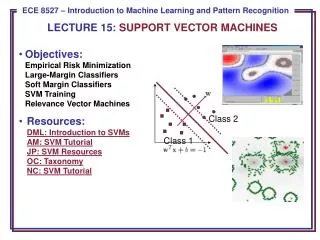
OUTLINE Margin-based loss - Example: binary classification - VC-theoretical motivation - Philosophical motivation SVM for classification SVM examples Support Vector regression SVM and regularization Summary
Given: Linearly separable data How to construct linear decision boundary? Example: binary classification
LDA solution Separation margin Linear Discriminant Analysis
All solutions explain the data well (zero error) All solutions ~ the same linear parameterization Larger margin ~ more confidence (~ falsifiability) Largest-margin solution
VC Generalization Bound and SRM • Classification:the following bound holds with probability of for all approximating functions where is called the confidence interval • Two general strategies for implementing SRM: 1. Keep fixed and minimize (most statistical and neural network methods) 2. Keep fixed (small) and minimize recall examples shown earlier: larger margin smaller VC-dimension
Complexity of -margin hyperplanes • If data samples belong to a sphere of radius R, then the set of -margin hyperplanes has VC dimension bounded by • For large margin hyperplanes, VC-dimension controlled independent of dimensionality d.
Motivation: philosophical • Classical view: good model explains the data + low complexity • Occam’s razor (complexity ~ # parameters) • VC theory: good model explains the data + low VC-dimension ~ VC-falsifiability: good model: explains the data + has large falsifiability The idea: falsifiability ~ empirical loss function
Adaptive loss functions • Both goals (explanation + falsifiability) can encoded into empirical loss function where - (large) portion of the data has zero loss - the rest of the data has non-zero loss, i.e. it falsifies the model • The trade-off (between the two goals) is adaptively controlled adaptive loss fct • Examples of such loss functions for different learning problems are shown next
Margin-based loss for classification: margin is adapted to training data
Margin based complexity control • Large degree of falsifiability achieved by - large margin (classification) - small epsilon (regression) • Margin-based methods control complexity independent of problem dimensionality • The same idea can be used for other learning settings
Single Class Learning Boundary is specified by a hypersphere with center a and radius r. An optimal model minimizes the volume of the sphere and the total distance of the data points outside the sphere
Margin-based loss: summary • Classification: falsifiability controlled by margin • Regression: falsifiability controlled by • Single class learning: falsifiability controlled by radius r NOTE: the same interpretation/ motivation for margin-based loss for different types of learning problems.
OUTLINE Margin-based loss SVM for classification - Linear SVM classifier - Inner product kernels - Nonlinear SVM classifier SVM examples Support Vector regression SVM and regularization Summary
( ) D x > + 1 1 w ( ) D x = + 1 ( ) D x ¢ w ( ) < - 1 D x ( ) D x = 0 x ¢ ( ) D x = - 1 Optimal Separating Hyperplane Distance btwn hyperplane and sample Margin Shaded points are SVs
Optimization Formulation Given training data Find parameters of a linear hyperplane that minimize under constraints Quadratic optimization with linear constraints tractable for moderate dimensions d For large dimensions use dual formulation: - scales with n rather than d - uses only dot products
From Optimization Theory: For a given convex minimization problem with convex inequality constraints there exists an equivalent dual unconstrained maximization formulation with nonnegative Lagrange multipliers Karush-Kuhn-Tucker (KKT) conditions: Lagrange coefficients only for samples that satisfy the original constraint with equality ~ SV’s have positive Lagrange coefficients
Convex Hull Interpretation of Dual Find convex hulls for each class. The closest points to an optimal hyperplane are support vectors
Dual Optimization Formulation Given training data Find parameters of an opt. hyperplane as a solution to maximization problem under constraints Note:data samples with nonzero are SVs Formulation requires only inner products
( ) x = 1 - D x 1 1 x 1 ( ) x 1 - D x = 2 2 x 2 ( ) D x + 1 = x 3 ( ) D = x 0 ( ) x = + D x 1 3 3 ( ) D x - = 1 SVM for non-separable data Minimize under constraints
SVM Dual Formulation Given training data Find parameters of an opt. hyperplane as a solution to maximization problem under constraints Note:data samples with nonzero are SVs Formulation requires only inner products
Nonlinear Decision Boundary • Fixed (linear) parameterization is too rigid • Nonlinear curved margin may yield larger margin (falsifiability) andlower error
Nonlinear Mapping via Kernels Nonlinear f(x,w) + margin-based loss = SVM • Nonlinear mapping to feature z space, i.e. • Linear in z-space=nonlinear in x-space • BUT ~ kernel trick Compute dot product via kernel analytically
SVM Formulation (with kernels) Replacing leads to: Find parameters of an optimal hyperplane as a solution to maximization problem under constraints Given:the training data an inner product kernel regularization parameter C
Examples of Kernels Kernel is a symmetric function satisfying general (Mercer’s) conditions Examples of kernels for different mappings xz • Polynomials of degree q • RBF kernel • Neural Networks for given parameters Automatic selection of the number of hidden units (SV’s)
More on Kernels • The kernel matrix has all info (data + kernel) H(1,1) H(1,2)…….H(1,n) H(2,1) H(2,2)…….H(2,n) …………………………. H(n,1) H(n,2)…….H(n,n) • Kernel defines a distance in some feature space (aka kernel-induced feature space) • Kernels can incorporate apriori knowledge • Kernels can be defined over complex structures (trees, sequences, sets etc)
Kernel Terminology • The term kernel is used in 3 contexts: - nonparametric density estimation - equivalent kernel representation for linear least squares solution - SVM kernels • SVMs are often called kernel methods • Kernel trick can be used with any classical linear method, to yield a nonlinear method. For example, ridge regression + kernel LS SVM
Support Vectors • SV’s ~ training samples with non-zero loss • SV’s are samples that falsify the model • The SVM model depends only on SVs SV’s ~ robust characterization of the data WSJ Feb 27, 2004: About 40% of us (Americans) will vote for a Democrat, even if the candidate is Genghis Khan. About 40% will vote for a Republican, even if the candidate is Attila the Han. This means that the election is left in the hands of one-fifth of the voters. • SVM Generalization ~ data compression
New insights provided by SVM • Why linear classifiers can generalize? (1) Margin is large (relative to R) (2) % of SV’s is small (3) ratio d/n is small • SVM offers an effective way to control complexity (via margin + kernel selection) i.e. implementing (1) or (2) or both • Requires common-sense parameter tuning
OUTLINE Margin-based loss SVM for classification SVM examples Support Vector regression SVM and regularization Summary
SVM Classification Examples • Modified Iris data set - two input variables, petal length and petal width - binary classification, iris versicolor (+) and not () • Two SVM models: polynomial kernel and RBF kernel
Example SVM Applications • Handwritten digit recognition • Face detection in unrestricted images • Text/ document classification • Image classification and retrieval • …….
Handwritten Digit Recognition (mid-90’s) • Data set: postal images (zip-code), segmented, cropped; ~ 7K training samples, and 2K test samples • Data encoding: 16x16 pixel image 256-dim. vector • Original motivation: Compare SVM with custom MLP network (LeNet) designed for this application • Multi-class problem: one-vs-all approach 10 SVM classifiers (one per each digit)
Digit Recognition Results • Summary - prediction accuracy better than custom NN’s - accuracy does not depend on the kernel type - 100 – 400 support vectors per class (digit) • More details Type of kernel No. of Support Vectors Error% Polynomial 274 4.0 RBF 291 4.1 Neural Network 254 4.2 • ~ 80-90% of SV’s coincide (for different kernels) • Reduced-set SVM(Burges, 1996) ~ 15 per class
Face detection in images (Osuna, et al, 1997) • Goal: Detect and locate face(s) in an image • Training data: face and non-face 19X19 pixel images obtained from real data • Test: Set A313 high-quality images with 1 face Set B 23 mixed quality images ( multiple faces) • Preprocessing: illumination gradient correction, histogram equalization • Face Search Strategy: divide an image into overlapping sub-images, at multiple scales, and classify each sub-image using SVM • Multiple scales of the original image are used 5 million sub-images (for Set A)
Face detection: results • SVM Classifier: 2-nd order polynomial • Performance Results Detection rate False Alarm Test Set A 97% 4% Test Set B 74% 20%
Document Classification (Joachims, 1998) • The Problem: Classification of text documents in large data bases, for text indexing and retrieval • Traditional approach: human categorization (i.e. via feature selection) – relies on a good indexing scheme. This is time-consuming and costly • Predictive Learning Approach (SVM): construct a classifier using all possible features (words) • Document/ Text Representation: individual words = input features (possibly weighted) • SVM performance: • Very promising (~ 90% accuracy vs 80% by other classifiers) • Most problems are linearly separable use linear SVM
Understanding SVM Classifier Univariate histogram (for linear SVM) - Red ~ negativeBlue ~ positive Shows distribution of training data relative to decision boundary(0) and margins(-1/+1)
OUTLINE Margin-based loss SVM for classification SVM examples Support Vector regression SVM and regularization Summary
Linear SVM regression Assume linear parameterization SVM regression functional: where
Direct Optimization Formulation Given training data Minimize Under constraints
Dual Formulation for SVM Regression Given training data And the values of Find coefficients which maximize Under constraints
Example:regression using RBF kernel RBF estimate (dashed line) using SVM model uses only 6 SV’s (out of the 40 points)
Example: decomposition of RBF model Weighted sum of 6 RBF kernel fcts gives the SVM model