Hyperspectral Remote Sensing
Hyperspectral Remote Sensing. Lecture 12 prepared by R. Lathrop 4/06. How plant leaves reflect light. Graphics from http://landsat7.usgs.gov/resources/remote_sensing/radiation.php. Reflectance from green plant leaves.

Hyperspectral Remote Sensing
E N D
Presentation Transcript
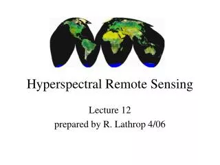
Hyperspectral Remote Sensing Lecture 12 prepared by R. Lathrop 4/06
How plant leaves reflect light Graphics from http://landsat7.usgs.gov/resources/remote_sensing/radiation.php
Reflectance from green plant leaves • Chlorophyll absorbs in 430-450 and 650-680nm region. The blue region overlaps with carotenoid absorption, so focus is on red region. • Peak reflectance in leaves in near infrared (.7-1.2um) up to 60% of infrared energy per leaf is scattered up or down due to cell wall size, shape, leaf condition (age, stress, disease), etc. • Reflectance in Mid IR (2-4um) influenced by water content-water absorbs IR energy, so live leaves reduce mid IR return
Hyperspectral Sensing • Multiple channels (50+) at fine spectral resolution (e.g., 5 nm in width) across the full spectrum from VIS-NIR-MIR to capture full reflectance spectrum and distinguish narrow absorption features
Hand-held Spectroradiometer • Calibrated vs “dark” vs. “bright” reference standard provided (spectralon white panel - #6 in image) • Can use “passive” sensor to record reflected sunlight or “active” illuminated sensor clip (#4)
Compact Airborne Spectrographic Imager (CASI) • Hyperspectral: 288 channels between 0.4-0.9 mm; each channel 0.018mm wide • Spatial resolution depends on flying height of aircraft and number of channels acquired CASI 550 For more info: www.itres.com
EO-1: Hyperion • The Hyperion collects 220 unique spectral channels ranging from 0.357 to 2.576 micrometers with a 10-nm bandwidth. • The instrument operates in a pushbroom fashion, with a spatial resolution of 30 meters for all bands. • The standard scene width is 7.7 kilometers. Standard scene length is 42 kilometers, with an optional increased scene length of 185 kilometers • More info: http://eo1.usgs.gov/hyperion.php
EO-1 • ALI & Hyperion designed to work in tandem
Hyperion over New Jersey EO1H0140312004120110PY_PF1_01 2004/04/29, 0 to 9% Cloud Cover EO1H0140312004120110PY_PF1_01 2004/04/29, 0 to 9% Cloud Cover EO1H0140312004120110PY_PF1_01 2004/04/29, 0 to 9% Cloud Cover EO1H0140312004184110PX_SGS_012004/07/02, 10% to 19% Cloud Cover EO1H0140312004184110PX_SGS_012004/07/02, 10% to 19% Cloud Cover
Hyperion Image EO1H0140312004120110PY 2004/04/29 R 800- G 650- B 550 Fallow field Active crop
Hyperion Image EO1H0140312004184110PX 2004/07/02 R 800- G 650- B 550 Conifer forest Deciduous forest
Hyperspectral Sensing: Analytical Techniques • Data Dimensionality and Noise Reduction: MNF • Ratio Indices • Derivative Spectroscopy • Spectral Angle or Spectroscopic Library Matching • Subpixel (linear spectral unmixing) analysis
Minimum Noise Fraction (MNF) Transform • MNF: 2 cascaded PCA transformations to separate out the noise from image data for improved spectral processing; especially useful in hyperspectral image analysis • 1st: is based on an estimated noise covariance matrix to de-correlate and rescale the noise in the data such that the noise has unit variance and no band-to-band correlation • 2nd: create separate a) spatially coherent MNF eigenimage with large eigenvalues (high information content, l>1) and b) noise-dominated eigenimages (l close to = 1)
MNF Transform: example 1 Plot of eigenvalue number vs. eigenvalue MNF 6 = noise Original TM image using ENVI software
MNF Transform: example 1 MNF 1 MNF 2 MNF 3 MNF 4 MNF 5 MNF 6
MNF Transform: example 2 Plot of eigenvalue number vs. eigenvalue MNF 5,6 7 = noise Tm_oceanco_95sep04.img Original TM image using ENVI software
MNF Transform: example 2 MNF 1 MNF 2 MNF 3 MNF 7 MNF 4 MNF 5 MNF 6
Plant Absorption Spectrum Image adapted from: http://fig.cox.miami.edu/~cmallery/150/phts/spectra.gif
Hyperspectral Vegetation Indices • NDVI = (R800 – R680) / (R800 + R680) at 680 (R800 – R705) / (R800 + R705) at 705 Where 680nm and 705nm are chlorophyll absorption maxima and 800 is NIR reference wavelength. 705nm may be more sensitive to red edge shifts
Hyperspectral Vegetation Indices • Photochemical Reflectance Index (PRI) designed to monitor the diurnal activity of xanthophyll cycle pigments and the diurnal photosynthetic efficiency of leaves • PRI = (R531 – R570) / (R531 + R570) where 531nm is the xanthophyll cycle wavelength and 570nm is a reference wavelength (Gamon et al., 1990, Oecologia 85:1-7)
Hyperspectral Water Stress Indices • Water Band Index (WBI) designed to monitor the vegetation canopy water status (Penuelas et al., 1997, IJRS 18:2863-2868) • WBI = R970 / R900 where 970nm is the trough in the reflectance spectrum of green vegetation due to water absorption (trough tends to disappear as canopy water content declines) and 900nm is a reference wavelength
Hyperspectral Water Stress Indices • Moisture Stress Index (MSI) contrast water absorption in the MIR with vegetation reflectance (leaf internal structure) in the NIR • MSI: MIR / NIR or R1600/R820 • Normalized Difference Water Index NDWI: (R860-R1240) / (R860+R1240)
Detection of Xylella fastidiosa Infection ofAmenity Trees Using Hyperspectral ReflectanceGH Cook project by Bernie Isaacson Cook 2006
Hyperspectral reflectance curves Green – not scorched yellow – scorching brown - senesced
Normalized Difference Vegetation Index at 680nm modified Photochemical Reflectance Index Photochemical Reflectance Index Simple Ratio Normalized Difference Vegetation Index at 705nm Red wavelengths to Green wavelengths Photosynthetic Active Radiation modified Water Band Index Water Band Index Hyperspectral Indices Applied
X - denotes significant difference Negative vs. Symptomatic Positive (Margins and Bases) l - denotes significant difference not detected Red text - denotes N<10 Negative vs. Symptomatic Positive (Margins Only)
Pre-Visual Stress Detection? • Hypothesis: Change in reflectance detectable before visual symptoms • Where can symptoms be detected? • Infected vs. Uninfected • Symptomatic (showing scorch) vs. Asymptomatic (tree infected but no symptoms) Slide adapted from B. Isaacson
Derivative Spectroscopy • First order: quantify slope, the rate of change in spectra curve • Second order: identify slope inflection points • Third order: identify maximum or minimum • Pros: can be insensitive to illumination intensity variations • Con: sensitive to noise
Derivative Spectroscopy: Blue Shift of Red Edge As chlorophyll degrades, less absorption in the red. Leads to a shift in the ‘Red Edge’ (i.e., between 690 and 740nm) towards the blue Stressed plant %R Blue Shift ‘Red Edge’ inflection point Normal plant Spectral wavelength
Original spectral reflectance profile 1st derivative The derivative is the slope of the signal: Derivative positive (+) signal slope increasing Derivative = 0 slope = 0 Derivative negative (-) signal slope decreasing 2nd derivative Graphic from http://www.wam.umd.edu/~toh/spectrum/Differentiation.html
Derivative spectroscopy • Red Edge inflection point (point where the slope is maximum) at the center of the 690-740nm range • Corresponds to the maximum in the 1st derivative • Corresponds to the zero-crossing (point where the signal crosses the y = 0 line going either from positive to negative or vice versa) in the second derivative
Spectra Matching • Spectra Matching: takes an atmospherically corrected unknown pixel and compares it to reference spectra • Reference spectra determined from: • In situ or lab spectro-radiometer measurements • Spectral image end-member analysis • Theoretical calculations • Number of different matching algorithms
Spectra Matching: spectral libraries USGS Digital Spectral Library covers the UV to the NIR and includes samples of mineral, rocks, soils, vegetations, microorganism and man-made materials http://speclab.cr.usgs.gov/spectral-lib.html Nicolet spectrometer
From http://speclab.cr.usgs.gov Reference spectra used in the mapping of vegetation species. The field calibration spectrum is from a sample measured on a laboratory spectrometer, all others are averages of several spectra extracted from the AVIRIS data. Each curve has been offset from the one below it by 0.05.
The continuum-removed chlorophyll absorption spectra from Figure 1 are compared. Note the subtle changes in the shapes of the absorption between species. From http://speclab.cr.usgs.gov
Spectral matching: Spectral Angle Mapper Material 1 Band Y Reference material Material 2 Band X Spectral Angle Mapper: computes similarity between unknown and reference spectra as an angle between 0 and 90 (or as cosine of the angle). The lower the angle the better the match.
Subpixel Analysis:Unmixing mixed pixels Spectral endmembers: signature of “pure”land cover class endmember1 Unknown pixel represents some proportion of endmembers based on a linear weighting of spectral distance. For example: 60% endmember 2 20% endmember 1 20% endmember 1 Band j unknown pixel endmember3 endmember2 Band i
Water Colora function of organic and inorganic constituents • Suspended sediment/mineral: brought into water body by erosion and transport or wind-driven resuspension of bottom sediments • Phytoplankton: single-celled plants also cyanobacteria • Dissolved organic matter (DOM): due to decomposition of phytoplankton/bacteria and terrestrially-derived tannins and humic substances
Ocean Color Spectra Open Ocean Coastal Ocean Red Algae bloom
Water Colora function of organic and inorganic constituents • Phytoplankton: contain photosynthetically active pigments including chlorophyll a which absorbs in the blue (400-500nm) and red (approx. 675nm) spectral regions; increase in green and NIR reflectance • Suspended sediment and DOM will confound the chlorophyll signal. Typical occurrence in coastal or Case II waters as compared to CASE I mid-ocean waters
Ocean Color: function of chlorophyll and other phytoplankton pigments Typical reflectance curve for CASE 1 waters where phytoplankton dominant ocean color signal. Arrow shows increasing chlorophyll concentration, dashed line clear water spectrum. Adapted from Robinson, 1985. Satellite Oceanography 100 10 %R 1 0 400 500 600 700 nm
Water Colora function of organic and inorganic constituents • Suspended sediment/minerals: increases volumetric scattering and peak reflectance shifts toward longer wavelengths as more suspended sediments are added • Near IR reflectance also increases • Size and color of sediments may also affect the relative scattering in the visible
Water Colora function of organic and inorganic constituents • Dissolved organic matter DOM: strongly absorbs shorter wavelengths (e.g., blue) • High DOM concentrations change the color of water to a ‘tea-stained’ yellow-brown color
Ocean Color RS Sensors: CZCS, SeaWiFS & MODIS Higher spectral resolution bands across the visible, with concentration in blue and green Example: CZCS wavebands Bands 1-6 have 20 nm bandwidth; bands 7 and 8 have 40 nm bandwidth. http://daac.gsfc.nasa.gov/CAMPAIGN_DOCS/OCDST/what_is_ocean_color.html