Download
1 / 26
260 likes | 388 Vues
US IOOS Modeling Testbed Leadership Teleconference May 3, 2011. Estuarine Hypoxia Team Carl Friedrichs, VIMS cfried@vims.edu 804-684-7303. Outcomes and Scientific Insights Gained. 5 Hydrodynamic Models Run for 2004:. (1) CH3D (C. Cerco/L. Linker, USACE/EPA/CBP). (2) EFDC

E N D
US IOOS Modeling TestbedLeadership TeleconferenceMay 3, 2011 Estuarine Hypoxia Team Carl Friedrichs, VIMS cfried@vims.edu 804-684-7303
Outcomes and Scientific Insights Gained 5 Hydrodynamic Models Run for 2004: (1) CH3D (C. Cerco/L. Linker, USACE/EPA/CBP) (2) EFDC (J. Shen/B. Hong, VIMS) ~ 18,000 wet grid cells ~ 54,000 wet grid cells
Outcomes and Scientific Insights Gained (cont.) 5 Hydrodynamic Models Run for 2004 (cont.): (4) UMCES ROMS (M. Li/J. Li, UMCES) ~20,000 wet cells (3) ChesROMS (R. Hood/W. Long, UMCES) ~5000 wet cells (5) CBOFS2 ROMS (L. Lanerolle, NOAA-CSDL) ~20,000 wet cells
Outcomes and Scientific Insights Gained (cont.) Six DO-Hydrodynamic combinations compared so far for 2004: (1) ICM: Complex biology w/CH3D (C. Cerco/L. Linker – USACE/EPA/CBP) (2) ChesROMS-bgc: NPZD biogeochemical model (W. Long/R. Hood – UMCES) (3) EFDC-1eqn: Simple DO model with SOD (J. Shen/B. Hong – VIMS) (4) CBOFS-1term: Constant net respiration (L. Lanerolle – NOAA-CSDL) (5) ChesROMS-1term: Constant net respiration (M. Scully – ODU) (6) ChesROMS-1DD: Depth-dependent net respiration (M. Scully – ODU)
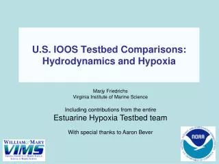
Outcomes and Scientific Insights Gained (cont.) Data set for model skill assessment: ~ 40 EPA Chesapeake Bay stations Each sampled ~ 20 times in 2004 Temperature, Salinity, Dissolved Oxygen Map of Late July 2004 Observed Dissolved Oxygen [mg/L] (http://earthobservatory.nasa.gov/Features/ChesapeakeBay)
Outcomes and Scientific Insights Gained (cont.) Metric for model skill assessment: Target diagram analysis (modified from M. Friedrichs)
Outcomes and Scientific Insights Gained (cont.) Five hydrodynamic models, today’s example parameters: -- bottom temperature -- bottom salinity -- maximum stratification (dS/dz) Six dissolved oxygen models, today’s example parameters: -- bottom DO, including model performance at individual stations -- hypoxic volume, including model performance in time
Outcomes and Scientific Insights Gained (cont.) Results: Bottom Temperature (2004) inner circle: CH3D (CBP model) outer circle: mean of data Models all successfully reproduce seasonal/spatial variability of bottom temperature (ROMS models do best) (M. Friedrichs, A. Bever)
Outcomes and Scientific Insights Gained (cont.) Results: Bottom Salinity (2004) CH3D mean of data Models all reasonably reproduce seasonal/spatial variability of bottom salinity (CH3D, EFDC do best) (M. Friedrichs, A. Bever)
Outcomes and Scientific Insights Gained (cont.) Results: Stratification (max dS/dz) mean of data Stratification is a challenge; CH3D, EFDC reproduce seasonal/spatial variability best (M. Friedrichs, A. Bever)
Outcomes and Scientific Insights Gained (cont.) Results: Bottom Dissolved Oxygen [Note: This does not evaluate ability to model year-to-year changes associated with yearly differences in nutrient input.] inner circle: ICM (complex CBP model) outer circle: mean of data Simple models reproduce seasonal/temporal variability in bottom DO about as well as ICM (M. Friedrichs, A. Bever)
Outcomes and Scientific Insights Gained (cont.) Results: Bottom Dissolved Oxygen – data from individual monitoring stations (normalized by individual station observed standard deviations) [mg/L] ICM (complex CBP model) ChesROMS with simple 1-term DO circle: mean of data 1-term DO model underestimates high DO and overestimates low DO: high not high enough, low not low enough (M. Friedrichs, A. Bever)
Outcomes and Scientific Insights Gained (cont.) Results: Hypoxic Volume [Note: This does not evaluate ability to model year-to-year changes associated with yearly differences in nutrient input.] inner circle: ICM (complex CBP model) outer circle: mean of data Several simple DO models reproduce seasonal variability of hypoxic volume about as well as ICM (M. Friedrichs, A. Bever)
Outcomes and Scientific Insights Gained (cont.) Results: Hypoxic Volume Time Series [Note: This does not evaluate ability to model year-to-year changes associated with yearly differences in nutrient input!] (spatially interpolated observations) Several simple DO models reproduce seasonal variability of hypoxic volume about as well as ICM (A. Bever)
Outcomes and Scientific Insights Gained (cont.) Analyses: Uncertainties in hypoxic volume observations and models Hypoxic Volume from CBP interpolated observations and ICM (complex) model In July 2004, ICM underestimates observed hypoxia at CBP stations, but difference between interpolated model results and integration of complete model results is ~ 5 km3 (A. Bever)
Outcomes and Scientific Insights Gained (cont.) Analyses: Uncertainties in hypoxic volume observations and models Hypoxic Volume from CBP interpolated observations and ICM (complex) model and ChesROMS-1DD (simple 1 term model) 1) Summer 2004 hypoxic volume from interpolation of observations: ~ 7.5 km3 2) Summer 2004 hypoxic volume from ICM: ~ 11 km3 3) Summer 2004 hypoxic volume from ChesROMS-1DD: ~ 8 km3 Spatial/temporal uncertainties in HV interpolations: ~ 5 km3 It’s not clear which of these three summer 2004 estimates is closest to the true value.
Outcomes and Scientific Insights Gained (cont.) Analyses: Effects of physical forcing on hypoxia – ChesROMS-1term Base Case Hypoxic Volume in km3 Jan Feb Mar Apr May Jun Jul Aug Sep Oct Nov Dec (by M. Scully) Date in 2004
Outcomes and Scientific Insights Gained (cont.) Analyses: Effects of physical forcing on hypoxia – ChesROMS-1term Base Case Hypoxic Volume in km3 Freshwater river input constant in time Jan Feb Mar Apr May Jun Jul Aug Sep Oct Nov Dec (by M. Scully) Date in 2004 Seasonal changes in hypoxia are not a function of seasonal changes in freshwater
Outcomes and Scientific Insights Gained (cont.) Analyses: Effects of physical forcing on hypoxia – ChesROMS-1term July wind year-round Base Case Hypoxic Volume in km3 Jan Feb Mar Apr May Jun Jul Aug Sep Oct Nov Dec (by M. Scully) Date in 2004 Seasonal changes in hypoxia may largely be due to seasonal changes in wind
Outcomes and Scientific Insights Gained (cont.) Analyses: Effects of physical forcing on hypoxia – ChesROMS-1term Base Case Hypoxic Volume in km3 January wind year-round Jan Feb Mar Apr May Jun Jul Aug Sep Oct Nov Dec (by M. Scully) Date in 2004 Seasonal changes in hypoxia may largely be due to seasonal changes in wind
Summarize Testbed Products Completed by June Broad-view Highlights of Key Products Completed by June • Intercomparison of skill for 5 CB Hydrodynamic models for all of 2004 • Sensitivity tests on these models (e.g., freshwater, ocean forcing, wind, horizontal and vertical grid resolution, vertical diffusivity) • Intercomparison of skill for 6 CB Hypoxia models for all of 2004 • Sensitivity tests on these models (e.g., freshwater, wind, vertical diffusivity) • Error bounds on hydrodynamic and DO models • Grids, forcings and output posted in NetCDF by Cyberinfrastructure Team • Workshop-based recommendations for EPA-CBP transition to new (multiple) hydrodynamic models (including draft of white paper for CBP) • “Alpha” transition of 1-term DO model for operational forecast use by NOAA-CSDL
Anticipated Progress During NCE (Jun-Dec) Broad-view Highlights of Example Progress Anticipated for NCE • Include all of 2005 in hydrodynamic and hypoxia modeling intercomparison • Include results from unstructured grid SELFE model in intercomparison • Assess effect of multi-model ensemble modeling on skill/error bounds • Finish configuration of multiple CB ROMS grids and forcings on single cluster at CSDMS for optimally controlled intercomparison/sensitivity tests • Collaborate with Cyberinfrastructure Team to preserve model output legacy • Relate results of MAB modeling to Chesapeake Bay conditions. • Complete white paper report for Chesapeake Bay Program on recommended transition to new/multiple hydrodynamic models • Present results at national science meetings • Submit papers, e.g., • C. Friedrichs et al. – Hydrodynamic model comparison to be published in ECM 2011 volume. • M. Friedrichs et al. – Hypoxia model comparison to be published in Biogeosciences (perhaps) • M. Scully et al. – Physical modulation of seasonal hypoxia in Chesapeake Bay • A. Bever et al. – Use of models to interpret errors in observations of Chesapeake Bay hypoxia • Estuarine & Shelf Hypoxia Teams – Comparison of hypoxia controls in CB vs. GoM
Challenges to Progress and Lessons Learned 1) Getting subs to do timely invoicing is a pain!
Challenges to Progress and Lessons Learned 2) Uncertainty about budget (asked to spend, spend, spend), then 6 month NCE. 3) Some trouble engaging the Middle Atlantic Bight modeling group. 4) It was good to have the team lead and those in charge of intercomparison not have a model “in the running”. 5) The openness of all participants, including Feds, was even better than we ever had expected. 6) Engagement of NOAA-CSDL and EPA/NOAA CBP was outstanding.
How Can TAEG Help You?How can SURA Mgmt Help You? -- TAEG/SURA continue to search for/push for options of follow up testbed projects/funding. -- Could SURA be the academic arm of the proposed NOAA-NCEP estuarine forecasting effort? -- SURA could lead the publication of cross-team overview articles, organize special sessions at national meetings, and special issues of journals. -- TAEG/SURA could help us plan how legacy tools/data will be preserved and made available to the community after the project is over.
Presentations at Scientific and Agency Meetings Presentations focused specifically on activities and results of Estuarine Hypoxia Team TestbedModelIntercomparison (i.e., as opposed to individual scientists’ own tangentially-related research projects) • Past Presentations: • 07/13/10 by C. Friedrichs at EPA/NOAA-CBP STAC Quarterly Meeting, Annapolis, MD. • 10/14/10 by C. Friedrichs at NSF CSDMS 2010 Meeting, San Antonio, TX. • 01/12/11 by C. Friedrichs at EPA/NOAA-CBP STAC Quarterly Meeting, Annapolis, MD. • 02/22/11 by A. Bever at EPA/NOAA-CBP DO Data Meeting, Annapolis, MD. • 03/23/11 by M. Friedrichs at EPA/NOAA-CBP STAC Quarterly Meeting, Annapolis, MD. • 04/05/11 by R. Hood at EPA/NOAA-CBP Modeling Subcommittee Meeting, Annapolis, MD. • Future Planned (so far) • Jun ‘11 by M. Friedrichs at CCMP Hydrodynamic Modeling Workshop, Edgewater, MD. • Jun ‘11 by A. Bever at GRC Coastal Ocean Modeling Conference, South Hadley, MA. • Nov ‘11 by C. Friedrichs at Estuarine & Coastal Modeling 2011, St. Augusting, FL. • Nov ‘11 by A. Bever at Coastal & Estuarine Research Federation, Daytona Beach, FL. • Feb ‘12 by M. Friedrichs at 2012 Ocean Sciences Meeting, Salt Lake City, UT.