Download
1 / 16
160 likes | 259 Vues
Information and guidelines for using the SPIRE II Spectrometer, including spectral coverage, observing modes, spectral resolutions, optical path differences, and spatial sampling options for effective observational planning.

E N D
Example Science Cases and AORs for SPIRE II. Spectrometer Nanyao Lu (NHSC/IPAC)
Covered Topics • Overview of the spectrometer and its observing modes. • HSpot demo: a single-pointing observation of the galaxy M82. • HSpot demo: a raster map observation of the extended galaxy M81. • Some considerations for your observational planning.
SPIRE Spectrometer Fourier Transform Spectrometer (FTS): The entire spectral coverage of 194-671 micron is observed in one go! (SMEC) (Not powered on; @4.5K)
From Interferogram to Spectrum Interferogram Source Spectrum Fourier Transform + Calibration Signal (volts) Optical path difference (cm)
Just One AOT! But a few Options • Low(0.83 cm-1; 25 GHz) • Medium (0.24 cm-1; 7.2 GHz) • High (0.0398 cm-1; 1.2 GHz) • What spectral resolution do you need? (set the FTS scanning distance) • Sparse (2 beam spacing) • Intermediate (1 beam spacing) • Full(1/2 beam, Nyquist) • What spatial sampling do you need? (set the number of BSM pointings) • Single point (1 FOV of 2’ in diameter) • Raster (NxM FOVs) • What is your source size? (set the number of telescope pointings)
High Spectral Resolution Medium Low Optical Path Difference 0 Spectral Resolutions Mode Δσ R Δv What for? High (HR) 0.04 cm-1 (1.2 GHz) 1290–370 230–800 km/s Line spectroscopy; Line detection & fluxes; Intermediate 0.24 cm-1 (7.2 GHz) 210–60 1410–4930 km/s Line detection & fluxes; (IR) Excitation studies; Low (LR) 0.83 cm-1 (25 GHz) 62–18 N/A Continuum High+Low Both HR & LR scans in the same observation. 12.8 cm Spectral resolution depends on the FTS scan distance.
Spectral Resolutions (Cont.) Blue curve: observed spectrum;Red curves: SINC function fits to CO lines.
SLW FWHM SSW FWHM Spatial Sampling Options Jiggling the beam-steering mirror (BSM) allows for 3 spatial sampling modes: Full Sparse Intermediate (half beam spacing) (1 beam spacing) (2 beam spacing) 16 point jiggle no jiggling 4 point jiggle Circle of 2’ diameter • Useful for larger maps • by sacrificing some • details. • Detailed mapping of an area • with Nyquist sampling. • Time consuming though. • For point source • observations. • Most economic.
Raster Maps • Raster map (< 30’x30’) is made of MxN identical individual fields • of view, each with a sparse, intermediate or full spatial sampling. • Step = 116 arcsec along raster rows • or 110 arcsec across rows. • Raster direction is fixed to spacecraft • axes. So check the entire visualization • range for adequate sky coverage, or • set a time constraint for the observation. • If necessary, may consider breaking up • a large map into smaller maps to save • time. 8x3 raster
Hspot Demo: A Single Pointing Observation of M82 Detailed time line when clicked
Hspot Demo: A Single Pointing Observation of M82 (Cont.) Panuzzo et al 2010
Hspot Demo: Raster Map Examples on M81 10’x5’ (6x4) raster on 29 April 2012. 10’x5’ (6x4) raster on 01 March 2012. Check representative map orientations over all possible future visibilities! If necessary/possible, make your map larger (thus, more costly), impose time constraints (thus, reducing chance for scheduling) or break a large map into smaller maps.
May Want to Break a Large Raster Map into Smaller Maps All using 4 FTS scan repeats, sparse sampling, high spectral resolution Two 6x6 rasters; Total time = 11.7 hr Two 6x6 rasters; Total time = 11.7 hr One 9x9 raster; Total time = 13.1 hrs (on 29 Apr 2012) (on 01 Mar 2012)
Good for line detection, but not ideal for resolving lines (e.g., suitable for gas excitation study). Very efficient for multiple line emission mapping (e.g., suitable for gas outflow or velocity field study). Telescope background (~ 500/1000 Jy in SSW/SLW) dominates. A photometer companion observation is highly recommended in cases of spectroscopy of a faint continuum (< a few Jy). Line spectroscopy is less affected by telescope background. On the other hand, if your target is (unfortunately) very bright (> 400/200 Jy for SSW/SLW; e.g., Galactic center), you may consider using the bright-source detector setting. Some Planning Considerations
For point source observations, it is best to place the target on the central detectors, which are still best calibrated at this point. Line blending could be a problem in hot molecular cores even with the high resolution mode. Even a small raster observation using high spectral resolution and full spatial sampling could be quite costly. If you can, a higher scan repetition is always desirable for better deglitching using scan redundancy (e.g., a repetition of 4 is better than 2). A large map with time constraints may make your observation not schedulable at all. You may want to break it into smaller maps. Some Planning Considerations (cont.)