Ocean data assimilation David Anderson
Ocean data assimilation David Anderson. Thanks to Magdalena Balmaseda, Patrick Vidard, Alberto Troccoli,Tim Stockdale. Outline of lecture. The ocean observing system The assimilation scheme and applications Salinity and altimetry Bias correction Future developments 3dVar, 4dVar, EnKF.

Ocean data assimilation David Anderson
E N D
Presentation Transcript
Ocean data assimilationDavid Anderson Thanks to Magdalena Balmaseda, Patrick Vidard, Alberto Troccoli,Tim Stockdale
Outline of lecture • The ocean observing system • The assimilation scheme and applications • Salinity and altimetry • Bias correction • Future developments 3dVar, 4dVar, EnKF
Why do we do ocean analyses • To provide initial conditions for seasonal forecasts. • To provide initial conditions for monthly forecasts • To provide initial conditions for multi-annual forecasts (experimental only at this stage) • To monitor the state of the ocean • We make regular ocean reanalyses covering more than 40 years, but data coverage is limited in early years.
The observing system • Moorings (Tao, PIRATA AND TRITON) (T) • XBTs (dropped from ships of opportunity) (T) • CTDs (High quality but very few- obtained by research ships) T and S • SST from satellite (IR,MW), ship and buoys. • SSS from a few ships, from a few moorings, from satellite in future. (eg SMOS, Aquarius) • Sea level from altimetry (ERS,TOPEX, Jason1, 2) • Current meters (very few ~5 along equatorial pacific) • Subsurface temperature and salinity from ARGO • (T=Temperature, S=Salinity, SST=Sea Surface Temperature, SSS=Sea Surface Salinity, IR=infrared, MW=micro-wave)
Atlas moorings are the backbone of the equatorial ocean observing system. They measure T at 10 depths from the surface to 500m. The data are transmitted via satellite and are on the GTS within a few hours.
Operating method of ARGO floats. Floats at 1000m for 10 days then rises to the surface measuring T and S as they rise. Measurements arethen transmitted by satellite. Some floats descend to 2000m before rising to the surface. • Operating
Distribution of 3000 floats. Upper on a regular grid (unachievable) and on a random distribution which might be more akin to what could be achieved.
Ocean data assimilationCURRENT SYSTEM-2 • The data assimilation is OI. • The window length is 10 days, with a 6 day delay for receipt of data. • No assimilation in the upper layer but there is a strong relaxation (~2days) to observed SST and a weaker relaxation to observed climatological SSS (Sea surface salinity). • Only T is analysed directly • Salinity and velocity are updated in physical space (rather than through covariances) • Analysis is done on model levels, one at a time.
Unlike the atmosphere, a great deal of information about the ocean state can be extracted from the forcing fields, in particular the tropical winds. • Ocean data can compensate for inaccurate winds, and model errors. • Any ocean analysis system therefore consists of forcing the ocean model as well as assimilating ocean data. • The forcing is needed for the previous several years as this is a typical adjustment time for the upper ocean. • In any event we want the ocean analyses to cover as many years as possible for (seasonal and monthly) forecast validation.
The background error covariance function is highly non isotropic to reflect the nature of equatorial waves- Equatorial Kelvin waves which travel rapidly along the equator ~2m/s but have only a limited meridional scale as they are trapped to the equator.
Example of ocean analysis EW section along the equator. Atlantic in rightmost panel, Pacific in the middle, Indian in left panel. NS sections also available on web. Most of the action is near the thermocline ~100-50m (also see later).
Temperature difference between assimilation and simulation. The assimilation is too warm near the equator. One might expect the OI to cool the model where it is too warm. Does it?
Mean temperature increment. This pattern does not look like the previous figure. Data assimilation is correcting for systematic error but not in an obvious way. Propagation, advection, data distribution all contribute, including a possible spurious circulation set up by the assimilation itself (see later).
Univariate data assimilation can be a problem • We have temperature data to assimilate but until recently, no salinity data. Velocity data remain scarce. • Unfortunately leaving salinity untouched can lead to instabilities. The following slide shows the problems that can occur if salinity is not corrected. A partial solution is to preserve the water-mass (T-S) properties below the surface mixed layer. In system-1, salinity was not corrected. It is corrected but not analysed in system-2. It is corrected and analysed in system-3. • The OI increments are spread uniformly throughout the assimilation window, to allow the model to spin-up its own velocity field.
Stratified Temp at I.C Temperature Temperature Spurious Convection Develops Salinity Salinity Meridional Sections (Y-Z) 30W 3 months into assimilation Constraint: To update salinity to preserve the water mass properties (Troccoli et al 2001)
So, by modifying S to conserve the model T-S profile, gross errors in S and T can be avoided, even though there are few measurements of S. Comparison of model sea level to altimetry shows that the fit in the Pacific is good and that in the Atlantic is improved but still not ideal.
How many analyses? • An ensemble of ocean analyses is created. • Five ocean analyses are created by perturbing the wind stress with perceived uncertainty. (These analyses are used to create an ensemble of forecasts.) The purpose of creating an ensemble of ocean analyses is to represent some of the uncertainty in knowing the ocean state. These analyses are used in creating the ensemble of forecasts in System-2 (the current ECMWF seasonal forecast system and in the monthly forecast system).
This plot shows a north-south section along 140W in the Pacific (upper) and the standard deviation of the temperature induced by the wind perturbations but controlled by data assimilation. Note the different scales. The variability (uncertainty) is not particularly small compared with the size of the signal.
ECMWF: Weather and Climate Dynamical Forecasts 10-Day Medium-Range Forecasts Seasonal Forecasts Monthly Forecasts Atmospheric model Atmospheric model Wave model Wave model Ocean model Real Time Ocean Analysis ~8 hours New Delayed Ocean Analysis ~11 days
t-11 days Heat,Wind stress, P-E Heat,Wind stress, P-E Ocean Analysis (seas) Obs-OI today Obs-OI Real time ocean analysis Real Time Ocean Analysis • Early delivery Ocean Analysis: • Used as I.C. for Monthly Forecasts • “Delayed” Ocean Analysis: • Used as I.C. of Seasonal Forecasts
The future • Later this year • We plan to implement an updated analysis system as part of System-3 • S assimilation • Altimeter assimilation • Bias correction • Different wind and temperature perturbations • Longer Term • Under development is a 3d and 4d var system. • These use the incremental approach as in meteorology. • In 4d var • a) Full nonlinear model is used for outer loops • b) An approximation to this is linearised • c) An exact adjoint to b) is generated • The cost function is quadratic and minimisation speeded up. • 5 inner loops to 1 outer loop
System-3 • Ocean model: HOPE (~1degx1deg, increasing to 1/3deg near the equator to resolve equatorially trapped waves such as the Kelvin wave) • Assimilation Method OI • Assimilation of T + Balanced relationships (T-S, ρ-U) • 10 days assimilation windows, increment spread in time • New Features • ERA-40 fluxes to initialize ocean • Retrospective Ocean Reanalysis back to 1959. • Multivariate on-line Bias Correction . • Assimilation of salinity data. • Assimilation of altimeter-derived sea level anomalies. • 3D OI
T/S conserved OI T/S Changed OI System 3: Assimilation of Salinity Observations • Motivations: • Known drift in salinity • S of T scheme improves S and T but not enough • Number of salinity data recently increased (ARGO) Idea: perform a second OI using T+S data to correct the T/S relationship (Haines et al 2005 ECMWF TECH Memo)
By analysing S on T surfaces, rather than z, we can spread the influence of data over larger distances, and so extract more information from the S data.
Altimetery • From satellites such as Topex, Jason and ERS, one can detect changes in the bending of the top surface of the ocean. This bending is small- in many places only a few cms, in some places up to ~30cms during El Nino for example. How to use this surface data to alter the density field beneath the surface?
The way it is done here is to displace the T-S profile vertically to match the sea-level. This preserves the T-S relation, which is a reasonable approximation throughout much of the water column but less likely to hold in the surface layer. Measurements of surface salinity would help. • Measurements of mean sea level would help to correct the mean state. Three satellites to help improve the mean sea level are in progress. (Two are already in orbit). GRACE, CHAMP, GOCE • Using a mean sea level from geodetic missions has proved difficult. So we have reverted to using the model mean state.
OI System3: Assimilation of Altimeter Data How to extract T/S information from Sea Level? How to combine Sea level and subsurface data? Cooper and Haines, 1999 Based on altimetry, we modify the model T and S. These are then used as background fields in an OI assimilating T and correcting S to preserve TS.
T/S conserved CH96 T/S conserved OI T/S Changed OI Assimilation of S(T) not S(z) Assimilation in the ECMWF operational system 3- Altimetry and salinity. Altimeter data are used first, then in situ S
Assimilation of Salinity Contribution To ENACT: Assimilation of salinity along T surfaces (TM #458, Haines et al MWR) and are orthogonal Nice property:
Data coverage for June 1982 Data coverage for Nov 2005 Changing observing system is a challenge for consistent reanalysis Today’s Observations will be used in years to come • ▲Moorings: SubsurfaceTemperature • ◊ ARGO floats: Subsurface Temperature and Salinity • + XBT : Subsurface Temperature
North Atlantic: T300 anomaly North Atlantic: S300 anomaly Climate Signals…. …or spurious trends due to changing observing system?
Salinity Trend in North Atlantic Without ARGO, the salinity trend is half the size ALL NO_ALTI NO_ARGO NEITHER
ECMWF participated in the EU project ENACT • This involved multi model, multi method, multi-annual ocean reanalysis. • The data are freely available for anyone interested
ENACT Multi-model, multi assimilation methods ocean reanalysis
For the Nino3 region in the equatorial east Pacific, most analyses agree on the T; the intermodel variation is small compared to the signal. For salinity this is not true.
The Ensemble Kalman Filter (EnKF) • The advantage of the EnKF approach is that it is based on the full nonlinear equations. No linearizations or closure assumptions are needed as for the extended Kalman filter and no adjoint equations are needed as for 4d var. • The EnKF will be tested at ECMWF in the coming year using a global ocean GCM. The size of the ensemble will be ~100. Is this big enough? This work is part of the ENSEMBLES project of the EU.
ENSEMBLE KALMAN FILTERING The equation for EnKF looks just like OI except A, D are matrices. Typically A would be n x N where n is the dimension of model space and N is the size of the ensemble (~100). An SVD of the first bracketed term allows for practical solution of this equation.
Some references related to ocean data assimilation at ECMWF • Ocean data assimilation for seasonal forecasting. D Anderson in ECMWF Seminar Proceedings Sept 2000. • Three and four dimensional variational assimilation with a general circulation model of the tropical Pacific. Weaver, Vialard, Anderson and Delecluse. ECMWF Tech Memo 365 March 2002. See also Monthly Weather Review 2003, 131, 1360-1378 and MWR 2003, 131, 1378-1395. • Balanced ocean data assimilation near the equator. Burgers et al J Phys Ocean, 32, 2509-2519. • Salinity adjustments in the presence of temperature adjustments. Troccoli et al Monthly weather rev 130, 89-102. • Comparison of the ECMWF seasonal forecast Systems1 and 2.. Anderson et al ECMWF Tech Memo 404. • Sensitivity of dynamical seasonal forecasts to ocean initial conditions. Alves, Balmaseda, Anderson and Stockdale. Tech Memo 369. Quarterly Journal Roy Met Soc. 2004. February 2004 • Recent developments in data assimilation for atmosphere and ocean. ECMWF Seminar Sept 2003. See Balmaseda and Weaver articles. • An ensemble Kalman smoother for nonlinear dynamics. Evensen and van Leeuwen Mon Weather Rev 128, 1852-1867. • The ensemble Kalman filter: theoretical formulation and practical implemenation. Evensen. Ocean Dynamics 2003. 53, 343-367. • Salinity assimilation usinf S(T) relationships. K Haines et al Tech Memo 458. Mon Wea Rev in press.