Download
1 / 27
270 likes | 302 Vues
Learn the fundamentals of Bayes' decision theory in statistical pattern recognition for optimal pattern classification. Explore the theory, formulas, rules, and decision surfaces to minimize misclassifications.

E N D
Statistical pattern recognition • The most popular approach to pattern classification • It has a firm background in mathematics (statistics) • It offers practically applicable solutions • It seeks to solve the classification task • Objects to be classified feature vectorx • Goal: to map each object (feature vector) into one of the classesC={c1,..,cM} • Background in statistics (probability theory): we will estimate the joint (conditional) probability of Xand C • Bayes’ formula: • P(ci|x) : thea posteriori probability of the ci class • P(x|ci) : theclass-conditional distribution of the xfeature vectors • P(ci) : thea priori distribution of the ci class • P(x) : it won’t be important for the optimal classification
The Bayes decision rule • We seek to minimize: the number (rate) of misclassifications on the long run • Formalization: Let’s introduce the 0-1 loss function i(ck,x) • Bayes’ decision rule: the long-run rate of misclassifications will be minimal if for each input vector x we chose the class ci for which P(ci|x) is maximal • Proof: we can formalize the error as the expected value of i(ck,x)We also call it the risk of chosing class ci: This will be minimal if P(ci|x) is maximal k: correct class i: selected class
The Bayes decision rule 2 • To calculate the global risk over all the feature space X we have to calculate • Of course, if we minimize the risk for all x values (i.e. we make an optimal decision for all x), then the global risk will also be minimized at the same time • The Bayes’ decision rule is a special case of what we called the indirect or decision theoretic approach earlier: • For each class ci we create the discriminant function gi(x)=P(ci|x) • We classify a test point x by selecting the class for which gi(x) is maximal • Note: this approach may also by used with other discriminant functions (e.g. using some heuristically selected functions). However, the proof guarantees optimality only for gi(x)=P(ci|x) • Using Bayes’ decision rule, the problem of classification boils down to estimating P(ci|x) from a finite set of data as accurately as possible
gi(x) ga(x) gb(x) a b Discriminant functions and decision surfaces • The discriminant functions together with the decision rules indirectly define decision surfaces. Example for two classes (a and b): • Note: certain transformations modify the discriminant functions, but not the decision boundary. E.g the following yield the same boundary (but may technically be easier or more difficult to handle):
P(x,i) P(x,i) c1 c1 c2 c2 R1 R1 R2 R2 The error of the Bayes’ decision • The probability of error for Bayes’ decision is visualized by the dashed area on the left figure for two classes (a and b): • Shifting the boundary would only increase the error (see fig. on the right) • The dashed area on the left figure is called the Bayes error • Given the actual distributions, this is the smallest possible error that can be achieved - But it might not be small on an absolute scale! • It can only be reduced by finding better features – i.e by reducing the overlap of the distributions of the classes
Probability estimation with discrete features • How can we estimate the distribution of discrete features? By simple counting • example: • P(joint_pain=yes|infuenza=yes)≈2/3 • P(joint_pain=no|infuenza=yes)≈1/3 • Simple counting work fine when the features has only a few values and we have a lot of examples. In other cases we might get unreliable estimates (there are many tricks to handle these cases…)
Prob. Estimation for continuous features • To apply Bayes’ decision theory, we have to find some way of modelling the distribution of our data. In the case of a continuous feature set we usually assume that the distribution can be described by some parametric curve. Using the normal (or Gaussian) distribution is the most common solution. • Univariate Gaussian distribution • Multivariate Gaussian distribution
Covariance matrix - Examples • We will visualize 2D densities using their contour lines
Covariance matrix - Examples • Diagonal covariance matrix with the same variance for both features • The contour lines are circles • Diagonal covariance matrix with different variances • Allows stretching the circles along the axes • Non-diagonal covariance matrix • Allows both stretching and rotation
Decision boundaries for normal distributions • For simplicity, let’s assume that we have only two classes • Let’s also assume that they can be described by normal distributions • The decision rule requires P(ci|x)=p(x|ci)P(ci)/p(x) • Here p(x) is constant for a given x, so it does not influence the maximum over i • The same is true for taking the logarithm • So we can use the discriminant function gi(x)=ln(p(x|ci)P(ci)) • where • Putting it all together gives
Special case #1 • Let’s assume that i=2I for both classes • Then We can discard: - det i , as it is the same for both classes, it does not influence the decision - -d/2 ln 2 is a constant, it does not influence the decision The remaining component reduces to: As 2 is independent of i, the disciminant function is basically is the euclidean distance to the mean vector of the classes
Special case #1 • How does the distributions and the decision surface look like in 2D? • Decomposing the discriminant functions, we get that • As xTx is independent of i, we can drop it. Then we get • This is a linear function of x, which means that the discriminant functionsare hyperplanes, and the decision boundary is a straight a line • We will discuss the role of P(ci) later
Special case #2 • i=, so the classes have the same (but arbitrary) covariane matrix Discarding the constans, the discriminant function reduces to The first term is known as the Mahalanobis distance of x and μi Decomposing the formula, we can drop xT-1x as it is independent of i So we get This is again linear in x, so the discriminant functions are hyperplanes, and the decision boundary is a straight a line
Special case #2 • Illustration in 2D
General case • The covariance matrices are different, and may take any form • In this case we cannot reduce the discriminant function, it remains quadratic in x. The decision boundary may take the shape of a conic section (line, circle, ellipsis, parabola or hyperbola). • Recommended reading: https://www.byclb.com/TR/Tutorials/neural_networks/ch4_1.htm
The effect of the class priors • HowdoesthedecisionboundarychangeifwechangeP(ci)? • g1(x)=p(x|c1)P(c1)g2(x)=p(x|c2)P(c2) • Don’tforgetthatP(c1) + P(c2)=1 • Changingthe ratio of P(c1) and P(c2)equalstomultiplyingthedisciminantfunctionsby a constant • Thiswill shift thedecisionboundarytowardsthe less frequentclass • P(c1)=0.5 P(c2)=0.5 P(c1)=0.1 P(c2)=0.9
The naïve Bayes classifier • We examined how the decision surfaces look like for Gaussian distributions with given parameters • What’s next?We will assume that the samples in each class have a Gaussian distribution (true or not, see later…) • And we will estimate the distribution parameters from the data • Our class distributions are of the form • So the parameters we have to estimate are μiand i for is each class ci • Don’t forget that x is a vector, so we have to estimate the parameters of a multivariate distribution! • As it is not an easy task, we start with a simplified model • This will be the naïve Bayes classifier
The naïve Bayes assumption • The naïve Bayes model assumes that the features are conditionally independent, so we can write • With this assumption, we have to estimate n 1-variable distributions instead of 1 n-variable distribution • This is mathematically and technically easier • For example we can use an univariate Gaussian distribution for a continuous feature • And we can estimate μ by the empirical mean of the data items: and σ2 by the empirical variance of the data over μ:(where D is the number of training examples) • We will prove later that these formulas are correct
The naïve Bayes model • A big advantage of the naïve Bayes model is that can easily handle the case when the feature vector consists of both discrete and continuous features! • For the discrete features we can apply a simple counting-based estimation, remember the example: • example: • P(joint_pain=yes|infuenza=yes)≈2/3 • P(joint_pain=no|infuenza=yes)≈1/3
The naïve Bayes model • The third advantage of the naïveBayes approach is that it is a very efficient tool against the curse of dimensionality • It is very useful when we have few training samples and/or a lot of features • Example: text classification with “bag of words” features • e-mails-> spam/notspam • Articles-> topic • … • We have to find some features that represent the text • “bag of words” representation: the number of the occurrence of each possible word in the text • Of course, the order of words is also important, but this is a very simple representation…
Example: the bag-of-words representation • This results if a HUGE feature space (100000 features) • For this task, any method other than Naïve Bayes is pretty difficult to use due to data sparsity (even if we have a lot of training data)
The naïve Bayes model - Summary • Advantages: • Mathematical simplicity, easy implementation • It can handle the mixture of continuous and discrete features • Very efficient in handling sparse data (large feature space, few samples) • Disadvantage: • Assuming feature independency is incorrect in most cases • In spite of this, the naïve Bayes approach is very popular and works surprisingly efficiently for many classification tasks
The sources of errors in statistical pattern recognition • In summary, creating a classifier by the statistical pattern recognition approach consists of 3 main steps: • Select a suitable feature set • Select a parametric model that we will use to describe the distribution of the data (when the features are continuous) • Based on a finite set of training data, estimate the parameter values of the model • The errors of these 3 steps all contribute to the final error of the classifier • Error = Bayes error + model error + estimation error • What can we do about it?
The sources of errors in statistical pattern recognition • Bayes error: If the features do not fully separate the classes, the class distributions will overlap • This will be present even if we perfectly know the distributions • The only way to decrease the Bayes error is to select different features • Model error: For mathematical tractability, we must assume something about the shape of the distribution (e.g. it is a Gaussian distribution) • The data rarely has this shape, there will be a mismatch – this is the error of the model choice • This error can be decreased by choosing a better model • Estimation error: we have to estimate the model parameters from the training data set via some training algorithm • This error can be decreased by using more training data and/or by refining the training algorithm