Download
1 / 34
340 likes | 564 Vues
Global Circulation Models – the basis for climate change science. Presented by James Reeler UWC. Weather prediction. Vilhelm Bierknes claimed we can predict weather by calculations. 7 equations that predicted "large-scale atmospheric motions.".

E N D
Global Circulation Models – the basis for climate change science Presented by James Reeler UWC
Weather prediction • Vilhelm Bierknes claimed we can predict weather by calculations. • 7 equations that predicted "large-scale atmospheric motions.". • Weather processes were too complex for calculation. • Computers became essential for this process. • NWP (National Weather prediction) first carried out by the Royal Swedish Air Force Weather Service in Stockholm (December 1954). • Forecasts were three times a week. • NWP was soon available in most western countries.
NWP vs climate models • NWPs are designed to predict regional weather conditions in the short (1-3 days) and medium (4-10 day) term. • Climate models are derived from these models, but are designed to predict weather conditions years into the future. • Given the moderate accuracy of models in the short term, how is it feasible to predict weather conditions so far into the future? • The answer is: STATISTICS. • Climate models are not designed to give an accurate forecast on a daily basis, but rather to predict means and variability in climatic indicators – to give a statistically accurate picture of CLIMATIC, not WEATHER conditions.
NWP vs climate models (cont) ContrastsNWPClimate models Goalto predict weatherto predict climate Spatial coverageregional or globalglobal Temporal rangedaysyears Spatial resolutionvariable (20-100km)usually coarse Relevance of: Initial conditionshighlow Clouds/radiationlowhigh Surface (land/ocean/ice)lowhigh Ocean dynamicslowhigh Modelstabilitylowhigh Time dimensionessentialignored
How does the climate work? • The global climate system is a result of the link of atmosphere, oceans, the ice sheets (cryosphere), living organisms (biosphere) and the soils, sediments and rocks (geosphere), each of which will be considered in greater detail after this. • Each of these systems is integrally connected to the others, and energy exchanges between and within systems, as well as other interactions (such as the provision of nuclei for rain droplet formation) determine climatic condtions. • However, despite the interconnectedness, an explanation must clearly focus on aspects separately, and the linkages between these systems. • Climate models allow us to study these aspects of the systems independently. • GCMs stitch these individual models together through a process of linkages, the development of which has taken many years and a great degree of understanding of the climate
The atmosphere I: vertical structure • The lowest level of the atmosphere (the troposphere) is where the majority of weather processes take place. • It contains 75% of the gases and almost all water vapour and aerosols. (Barry & Chorley,1992) • The tropopause marks the upper limit of the troposphere. • Temperature change is due to absorption of UV by the ozone layer. • Consequently very stable. • The atmosphere above this level is mostly irrelevant in terms of weather. • The action and feedbacks associated with clouds are still poorly understood, and only recently have models begun to incorporate cloud cover in any comprehensive detail. Source: Barry & Chorley, 1992
The atmosphere II: energy budget • 1368Wm-2 of incoming radiation hits the top of the atmosphere. • A black body would reflect all the radiation, although some would be absorbed and re-radiated as longer wavelengths (dotted lines). • However, atmospheric gases absorb some of the radiation, reducing the radiated energy (grey area). • Atmospheric gases/aerosols also scatter incoming radiation. • Although 30% of incoming energy is reflected, little of the remainder escapes directly. • The atmosphere consequently heats up (greenhouse effect). Source: IPCC Third Assessment Report
The atmosphere III: Horizontal transfers • Because of the earth’s curvature, more radiation falls in equatorial regions than at the poles. (Trewartha & Horn, 1980). • To restore equilibrium, an interchange of heat from tropics to poles occurs through movement of air masses. (Barry & Chorley, 1992) • This latitudinal transfer of energy occurs in several ways: • movement of sensible heat • movement of latent heat • ocean circulation Source: NASA • For each packet of air that moves polewards, a similar quantity moves towards the tropics, setting up circulation cells (also affected by the coriolis forces of the earth’s rotation). • These energy fluxes are the principal components of the climate – therefore actions which interfere with the fluxes necessarily affect the climate.
The oceans • It is divided into two distinct layers: • The upper, seasonal layer of warm mixed water that stretches up to 100m deep in the tropics, and interacts with the atmosphere. • The lower deeps, which contain more than 80% of the water in the oceans. • The ocean holds more energy than the atmosphere because: • Heat capacity is 4.2 times higher • Density is 1000 times higher. • Heat is transferred to the atmosphere by evaporation of water vapour, which passes on its energy to the atmosphere when it condenses into clouds or precipitates. • Vertical energy transfer at the poles – freezing oceans become more saline, and the water sinks. • The world therefore has extensive global thermohaline circulation, which warms polar regions and transfers nutrients to the tropics..
Biosphere • The biosphere is the living component of the world. It affects many aspects of the climate: • Plants absorb more light than bare ground, reducing albedo (coniferous forest: 0.09-0.15; cf. bare ground: 0.3). • The biosphere also affects the fluxes of certain greenhouse gases: - Terrestrial plants fix CO2 in their structure. - Oceanic plankton remove CO2 from the atmosphere as shells when they fall to the ocean bottom. • The biosphere also generates large amounts of aerosols such as spores, viruses, dust, bacteria and pollen that scatter and reflect incoming radiation. • Primary productivity in the oceans also generates dimethyl sulphides (DMS), which act as nuclei for cloud formation.
The geosphere • This is the physical structure of the earth, from the soils and rocks of the continental shelf to the planet’s core • The internal energies of the earth can cause climate change over extremely long periods. • Plate tectonics change the shape of the surface, and transform ocean basins or mountains, affecting energy transfers between coupled systems. • The structure of soil can affect both its interaction with the air (in terms of gas fluxes) and its water retention for biological processes. The Mahameruvolcano on the island Java of Indonesia. Photo by Jan-Pieter Nap • Volcanism can emit vast quantities of CO2 from single events, as well as putting large amounts of aerosols into the atmosphere, which can reduce incoming radiation for several years. (Sear et al., 1987).
Different types of climate models • It is often convenient to regard climate models as belonging to one of four main categories: • energy balance models (EBMs) • one dimensional radiative-convective models (RCMs); • two-dimensional statistical-dynamical models (SDMs) • three-dimensional general circulation models (GCMs). • It is not always necessary to use the most complex model. • Using a simpler model allows more runs to be carried out as sensitivity tests to assess the accuracy of modelling assumptions.
Energy balance models • These simple models only really concern themselves with two things: • Radiation balance (between incoming solar radiation and heat loss) • Latitudinal energy transfer • EBMs may be 0-D, in which case latitudinal characteristics are ignored. • In 1-D models, the dimension included is latitude. Temperature for each latitude band is calculated using the appropriate latitudinal value for the various climatic parameters
Radiative-convective models • These models are generally 1-D or 2-D, with height always present as a dimension. They model: • Radiative transformations as energy is absorbed, emitted and scattered. • The role of convection and vertical energy transfer through atmospheric motion. • By considering surface albedo, cloud amount and atmospheric turbidity, it calculates the heat absorption in various atmospheric layers. • If the heating in a layer exceeds a certain value (the lapse rate), it will convect into the layer above, transferring heat energy. • The tropical Hadley cells models are an example of this type of model. Source: http://www.newmediastudio.org/DataDiscovery/Hurr_ED_Center/Easterly_Waves/Trade_Winds/Trade_Winds_fig02.jpg
Statistical-dynamical models • These are generally 2-D, with one horizontal and one vertical dimension (although there are some models with two horizontal dimensions). • They combine the horizontal energy transfer of EBMs with the radiative-convective functions of RCMs. • However, the equator-pole transfer is more accurately simulated than in EBMs, based on theoretical and empirical relationships of the cellular flow between latitudes. • Energy diffusion is simulated using the laws of motion. • Statistical relationships define the windspeed and wind direction within the models. • These models are useful for simulating and studying horizontal energy flows, and processes that disrupt them. SOURCE: http://www.newmediastudio.org/DataDiscovery/Hurr_ED_Center/Easterly_Waves/Trade_Winds/Trade_Winds_fig01.jpg
Global circulation models • GCMs “…are the only credible tools currently available for simulating the response of the global climate system to increasing greenhouse gas concentrations” (IPCC-TGCIA, 1999). • The first GCM was a very simple 2 layer, hemispheric, quasi-geotrophic computer model, developed in the 1950’s by Norman Philips. • Such early GCMs involved several atmospheric layers and a very simple oceanic model. The model was run to equilibrium with a set CO2 level (such as 300ppm) and then the CO2 level was increased. • Contemporary models are considerably more complex, and are capable of being run in a transient mode. • They are 3-D, and may comprise thousands of individual cells
Contemporary GCMs: an outline • The most complex current models are known as coupled atmospheric ocean general circulation models (AOGCMs). • They have between 10 and 20 layers in the atmosphere, and as many as 30 layers in the ocean. • Contemporary AOGCMs have a horizontal resolution of between 250km and 600km. • For local planning, this is a very coarse scale, and the underlying topography is poorly represented. • However, taken over the whole globe, this resolution results in an extremely large number of individual cells. • For a given time step, calculations are carried out for each of these cells over the whole globe, including energy exchanges between each of the 26 adjacent cells. • Clearly this is very computationally intensive, and it is no surprise that atmospheric predictions have been at the forefront of computer development since the early 1950s.
DENSITY ADVECTION ADVECTION HEAT OF CONDENSATION HEATING AND COOLING MOISTURE SNOW COVER FEEDBACK PRECIPITATION HEAT ENERGY EVAPORATION Climatic processes modelled in a GCM Thermodynamic equation Equation of motion Equation of water vapour Radiation transfer Heat balance Hydrology of the earth’s surface
Flux adjustments • Some GCMs do not correctly provide a stable equilibrium condition under current climatic conditions. • In order to ensure they accurately do so, a number of “flux adjustments” are provided. • These are non-physical correction constants that are used as correction factors to ensure that the models stay on track. • More recently, through intensive exploration of more exacting physical calculations, some models have been developed that do not flux adjustments. • Some non-flux adjusted models are now able to maintain stable climatologies of comparable quality to flux adjusted models. • Furthermore, there is no systematic difference between the outputs of flux-adjusted and non-flux-adjusted models in terms of internal climatic variability.
How many GCMs are there? • Considering the incredible computing power necessary to run a full GCM, one would expect there to be only a few models. • In fact, a number of different groups have developed and refined models over the years, and the IPCC Third Assessment Report uses no fewer than 34 AOGCMs, some of which exist in several refinements. • These models are developed and operated by 18 different climatology centres, including the UK Meteorological Centre, National Center for Atmospheric Research, Goddard Institute for Space Studies and the Geophysical Fluid Dynamics Laboratory. • These models are run nearly constantly, and the results are published on the internet in order to allow planners and response modellers ready access.
Use of GCMs • GCMs enable us to better understand the processes that drive the climate. Models that work better at describing climatic conditions generally give us an insight into how the various physical characteristics of the earth are interacting. • They allow us to make informed and scientifically defensible predictions based on current understanding of the climate. • By running the models on palaeoclimatological data, an understanding of long-term climate effects far beyond the age of even the human race can be established. • GCMs are thus the best tools for all climate science, and allow conservationists, planners and politicians to test different response scenarios.
Climatic forcing • The effect of various factors on the climate are expressed as a forcing value (ie: to what extent they force global warming) • The forcing value is measured in Wm-2 (the increase in effective energy caused per square metre). • There are many natural forcing factors operating over different time periods, from desertification increasing albedo of a planet to the passage of the solar system through the galaxy (Williams, 1975). • Even the movements and placement of continents over time has some forcing activity. • However, these natural (also called external, or non-radiative) forcing factors are independent of those which directly affect the energy balance of the Earth-atmosphere (called radiative forcing factors) (Shine et al, 1990).
The effects of current radiative forcings Source: IPCC online slide archive
IPCC future scenarios • In order to predict future climate responses, the IPCC has modelled and detailed several different scenarios (IPCC, 1992; IPCC, 2000). • The SRES scenarios fall into four main “storyline” categories. • A1 – rapid economic growth and introduction of efficient technologies. • Global population peaks mid-century, then decreases. • Global capacity building; difference in per capita income between regions decreases. • Three separate sub scenarios depending on energy policy: • A1FI – fossil fuel intensive. • A1T – fossil fuel use phased out entirely. • A1B – balanced use of all sources ( no one dominates).
Development scenarios (cont). • A2 – very heterogenous world, focussed on self-reliance. • Constant population growth due to slow fertility rate change • Per capita economic and technological growth slow • Regional responses • B1 – similar population growth and global economy to scenario A1. • Rapid transition to service economies (low-impact) • Focus on provision of clean, resource efficient technology. • Global solutions to economic inequities, but no other climate initiatives. • B2 – emphasis on local solutions to economic, social, and environmental sustainability • Constant population growth (slower than A2). • Slower economic/social growth, focussed on a regional scale. • Focussed on environmental solutions and greater equity, but on a regional rather than global scale.
Future radiative forcings depend on response • Current climate change is largely anthropogenic in origin. • Human activities are likely to continue to affect the climate in a similar manner. • Consequently, the human political and economic response to global climate change is essential. • The SRES scenarios demonstrate how human response is likely to affect global greenhouse gas and aerosol emissions. Source: IPCC online slides
GCM model responses • All GCMs are tested to ensure that they correctly model previous palaeoclimatological conditions to the present day. • However, although they often agree on general trends for a given scenario, they may predict moderately different responses over time. • Consequently, climate scientists tend to use several different models and scenarios for any given set of predictions or plans. Click to enlarge • The IPCC TAR (Third Assessment Report) uses an average of as many as 20 model predictions when stipulating future climate trends, although as yet not all models have produced runs for all of the SRES future trend scenarios.
GCM outputs for 2100 (I) Source: IPCC online slides (SYR fig 3-3a &b)
Linear and non linear responses • Many climatic responses to changing conditions are linear in nature (either logarithmically through feedback mechanisms or as a flat line). • However, palaeoclimatological evidence points towards a number of periods of extremely rapid climate change. • This is typical of non-linear systems with multiple stable equilibria (Lorenz, 1993). • When conditions are pushed towards a “threshold value”, the transition to a new mode may be exceedingly rapid. • This has also been seen in recent changes in large scale circulation patterns detected by instrumental readings, and in contemporary observations of regional weather patterns. (Corti et al, 1999).
Examples of non-linear changes • Most GCMs show a slowing of the Atlantic Thermohaline Circulation as the world heats up. However, some show the circulation stopping entirely as heating reaches a threshold value. (Manabe and Stouffer, 1988). • Sea ice melting may be accelerated by feedback mechanisms. • Sea level rise may destabilise large polar ice masses, ice sheets, or even entire ice shelves, accelerating sea level rise. • Observed variability of ENSO indicate a transition to increased occurrence of ENSO in 1976, although not enough is know to say whether this is an anthropogenic effect, or even if it is a long-term transition. • Large-scale (possibly irreversible) transformations in the biosphere such as the growth of the Sahara desert (Claussen et al., 1999), have occurred even with minimal anthropogenic interaction. These can be seen as non-linear changes triggered by slow changes in forcing factors, and it seems highly possible that this could occur given the current level of anthropogenic disturbance. However, not enough is know about this incredibly complex system to say this with any degree of certainty.
Conclusion • General circulation models are the best tool we have for determining the range and extent of climate change, as well as for working out what is likely to happen in the future. • All current models agree that current climatic change is a result of anthropogenic influences. • Future climate change will depend on the current human response to that knowledge. • Although GCM outputs are very large scale, they can be refined and downscaled to assist in prediction for smaller areas. • Thus, the outputs from GCMs can be exceedingly useful in terms of conservation planning for responses to climate change.
Check your understanding of Chapter 2 PASS MARK 80% Please do not proceed further until you have PASSED Chapter 2: test yourself
Next Links to other chapters Chapter 1 The evidence for anthropogenic climate change Chapter 2Global Climate Models Chapter 3 Climate change scenarios for Africa Chapter 4 Biodiversity response to past climates Chapter 5 Adaptations of biodiversity to climate change Chapter 6 Approaches to niche-based modelling Chapter 7 Ecosystem change under climate change Chapter 8 Implications for strategic conservation planning Chapter 9 Economic costs of conservation responses I hope that found chapter 2 informative, and that you enjoy chapter 4. Chapter 3 has unfortunately been omitted for this course