Download
1 / 25
270 likes | 397 Vues
This research explores the efficiency optimization of induction motor drives, focusing on a dynamic programming approach to minimize energy consumption under specified operating conditions. Key findings reveal that adjusting the magnetizing flux can effectively reduce power losses. The study establishes an optimal control strategy that identifies the stator currents yielding minimal power losses for a given operating point. Comprehensive simulations and experimental tests validate the performance of the proposed model, emphasizing its applicability for enhancing energy efficiency in modern motor systems.

E N D
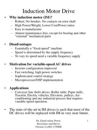
Presented by: Branko Blanu{a University of Banja Luka, Faculty of Electrical Engineering E-mail:bbranko@etfbl.net Research director: Prof. Slobodan N. Vukosavi}, Ph.D Niš 2007 Efficiency Optimization of Induction Motor Drive Based on Dynamic Programming Approach
Main goal: For a known operating conditions, define optimal control so the drive operates with minimal energy consumption
FUNCTIONAL APPROXIMATION OF THE POWER LOSSES IN THE INDUCTION MOTOR DRIVE.Inverter losses:where id , iq are components of the stator current in d,q rotational system and RINV is inverter loss coefficient.Motor losses:Main core losses:where yD is rotor flux, wesupply frequency and c1 andc2 are hystresis and eddy current loss coefficient.
Copper losses:where Rs is stator resistance, and Rr rotor resistance.Stray losses:The stray flux losses depend on the form of stator and rotor slots and are frequency and load dependent. The total secondary losses (stray flux, skin effect and shaft stray losses) must not exceed 5% of the overall losses-requirments of the EU for 1.1-90kW motors
Important conclusions 1. It is possible to minimize power losses by variation of magnetizing flux in the machine. 2. For a given working point of the induction motor, only one pair of the stator currents produce flux which gives minimum of the power losses. 3. For a known operating conditions and for closed-cycle operation, it is possible to define optimal control so the drive operates with minimal energy consumption
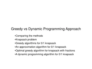
Optimal Control Computation Using Dynamic Programming Aproach In order to do that, it is necessary to define performance index, system equations, constraints and boundary conditions for control and state variablesand present them in a form suitable for computer processing 1. Performance index: (1) where N=T/Ts, T is a period of close-cycled operation and Ts is sample time. The L function is a scalar function of x-state variables and u-control variables, where x(i) , a sequence of n-vector, is determined by u(i), a sequence of m-vector
4. Boundary conditions x(0) has to be knownn 2. System equations 3. Constrains Equality contraints C[u(i)]=0 (Control variable equality constrains) C[x(i),u(i)]=0 (Equality constraints on function of control and state variables) S[x(i)]=0 (Equality constraints on function of state variables) Inequality contraints C[u(i)]0 (Control variable inequality constrains) C[x(i),u(i)] 0 (Inequality constraints on function of control and state variables) S[x(i)] 0 (Inequality constraints on function of state variables) i=0,1,..N-1
Following the above mentioned procedure, performance index, system equations, constraints and boundary conditions for a vector controlled induction motor drive in the rotor flux oriented reference frame, can be defined as follows 1. Performance index 2. System equation (dynamic of the rotor flux) where Tr=Lr/Rr is a rotor time constant
3. Constrains For torque Stator current Rotor speed Rotor flux 4. Boundary conditions Basically, this is a boundary-value problem between two points the boundary conditions of which are defined by starting and final value of state variables:
Following the dynamic programming theory , a system of differential equations can be defined as follows: (1) whereland m are Lagrange multipliers.
By solving the system of equations (1) and including boundary conditions, we come to the following system: (2)
Every sample time values of wr(i) and Tem(i) defined by operation conditions is used to compute the optimal control (id(i), iq(i), i=0,..,N-1) through the iterative procedure and applying the backpropagationrule, from stage i =N-1 down to stage i =0. Value of YD and have to be known. In this case, YD(N)=YDmin and
Simulation Results Operation conditions (speed reference and load torque ) are given in Fig. 1. and Fig. 2. Graph of power loss for given operation condition are presented in Fig. 3. Graph of power loss and speed response during transient process and for different methods are presented in Fig. 4. and 5.
Expermental results Experimental tests have been performed in the laboratory station for digital control of induction motor drives which consists of: - induction motor (3 MOT, D380V/Y220V, 3.7/2.12A, cosf=0.71, 1400o/min, 50Hz) - incremental encoder connected with the motor shaft, - three-phase drive converter (DC/AC converter and DC link), - PC and dSPACE1102 controller board with TMS320C31 floating pointprocessor and peripherals, - interface between controller board and drive converter.
Fig. 6 Graph of magnetization flux for LMC method a), dynamic programming approach b)
Fig. 7 Graph of mechanical speed for LMC method a), dynamic programming approach b)
Fig. 8 Graph of power loss for dynamic programming a), nominal flux b)
Conclusions 1. If load torque has a nominal value or higher in steady state, magnetization flux is also nominal regardless of whether an algorithm for efficiency optimization is applied or not. 2. At low loads in steady state, power loss for the LMC method and method based on dynamic programming is practically the same but significantly less than when the drive runs with nominal flux. 3.The method based on dynamic programming works in a way that magnetization flux starts to rise before the increase of load torque and keeps a higher value of magnetization flux during the transient processes than other methods for efficiency optimization. As a result, transient loss is lower and speed response is better.
4. The procedure of on-line parameter identification has been carried out in the background. In case the parameters change, a new optimal control value is computed for the next cycle of the drive operation. This increases the robustness of the algorithm in response to parameter variations. 5. Few simplifications in the computation of optimal control for the dynamic programming method have been made. Therefore, the computation time is significantly reduced. Some theoretical and experimental results show that some effects like nonlinearity of magnetic circuit for YDYDn has negligible influence in the calculation of optimal control. 6. One disadvantage of this algorithm is its off-line control computation.Yet, it is not complicated in terms of software. 7. This algorithm is applicable to different close-cycled processes of electrical drives, like transport systems, packaging systems, robots, etc.