Download
1 / 35
350 likes | 478 Vues
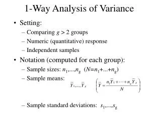
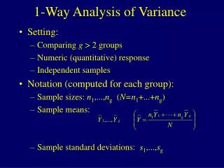
1-Way Analysis of Variance. Setting: Comparing g > 2 groups Numeric (quantitative) response Independent samples Notation (computed for each group): Sample sizes: n 1 ,..., n g ( N=n 1 +...+ n g ) Sample means: Sample standard deviations: s 1 ,..., s g. 1-Way Analysis of Variance.

E N D
1-Way Analysis of Variance • Setting: • Comparing g > 2 groups • Numeric (quantitative) response • Independent samples • Notation (computed for each group): • Sample sizes: n1,...,ng (N=n1+...+ng) • Sample means: • Sample standard deviations: s1,...,sg
1-Way Analysis of Variance • Assumptions for Significance tests: • The g distributions for the response variable are normal • The population standard deviations are equal for the g groups (s) • Independent random samples selected from the g populations
Within and Between Group Variation • Within Group Variation: Variability among individuals within the same group. (WSS) • Between Group Variation: Variability among group means, weighted by sample size. (BSS) • If the population means are all equal, E(WSS/dfW ) = E(BSS/dfB) = s2
Example: Policy/Participation in European Parliament • Group Classifications: Legislative Procedures (g=4): (Consultation, Cooperation, Assent, Co-Decision) • Units: Votes in European Parliament • Response: Number of Votes Cast Source: R.M. Scully (1997). “Policy Influence and Participation in the European Parliament”, Legislative Studies Quarterly, pp.233-252.
F-Test for Equality of Means • H0: m1 = m2 = = mg • HA: The means are not all equal • BMS and WMS are the Between and Within Mean Squares
Example: Policy/Participation in European Parliament • H0: m1 = m2 = m3= m4 • HA: The means are not all equal
Analysis of Variance Table • Partitions the total variation into Between and Within Treatments (Groups) • Consists of Columns representing: Source, Sum of Squares, Degrees of Freedom, Mean Square, F-statistic, P-value (computed by statistical software packages)
Estimating/Comparing Means • Estimate of the (common) standard deviation: • Confidence Interval for mi: • Confidence Interval for mi-mj:
Multiple Comparisons of Groups • Goal: Obtain confidence intervals for all pairs of group mean differences. • With g groups, there are g(g-1)/2 pairs of groups. • Problem: If we construct several (or more) 95% confidence intervals, the probability that they all contain the parameters (mi-mj) being estimated will be less than 95% • Solution: Construct each individual confidence interval with a higher confidence coefficient, so that they will all be correct with 95% confidence
Bonferroni Multiple Comparisons • Step 1: Select an experimentwise error rate (aE), which is 1 minus the overall confidence level. For 95% confidence for all intervals, aE=0.05. • Step 2: Determine the number of intervals to be constructed: g(g-1)/2 • Step 3: Obtain the comparisonwise error rate: aC= aE/[g(g-1)/2] • Step 4: Construct (1- aC)100% CI’s for mi-mj:
Interpretations • After constructing all g(g-1)/2 confidence intervals, make the following conclusions: • Conclude mi > mj if CI is strictly positive • Conclude mi < mj if CI is strictly negative • Do not conclude mimj if CI contains 0 • Common graphical description. • Order the group labels from lowest mean to highest • Draw sequence of lines below labels, such that means that are not significantly different are “connected” by lines
Example: Policy/Participation in European Parliament • Estimate of the common standard deviation: • Number of pairs of procedures: 4(4-1)/2=6 • Comparisonwise error rate: aC=.05/6=.0083 • t.0083/2,430 z.0042 2.64
Example: Policy/Participation in European Parliament Consultation Cooperation Codecision Assent Population mean is lower for consultation than all other procedures, no other procedures are significantly different.
Regression Approach To ANOVA • Dummy (Indicator) Variables: Variables that take on the value 1 if observation comes from a particular group, 0 if not. • If there are g groups, we create g-1 dummy variables. • Individuals in the “baseline” group receive 0 for all dummy variables. • Statistical software packages typically assign the “last” (gth) category as the baseline group • Statistical Model: E(Y) = a + b1Z1+ ... + bg-1Zg-1 • Zi =1 if observation is from group i, 0 otherwise • Mean for group i (i=1,...,g-1): mi = a + bi • Mean for group g: mg = a
Test Comparisons • mi = a+ bi mg = a bi = mi - mg • 1-Way ANOVA: H0: m1= =mg • Regression Approach: H0: b1 = ... = bg-1 = 0 • Regression t-tests: Test whether means for groups i and g are significantly different: • H0: bi = mi - mg= 0
2-Way ANOVA • 2 nominal or ordinal factors are believed to be related to a quantitative response • Additive Effects: The effects of the levels of each factor do not depend on the levels of the other factor. • Interaction: The effects of levels of each factor depend on the levels of the other factor • Notation: mij is the mean response when factor A is at level i and Factor B at j
Example - Thalidomide for AIDS • Response: 28-day weight gain in AIDS patients • Factor A: Drug: Thalidomide/Placebo • Factor B: TB Status of Patient: TB+/TB- • Subjects: 32 patients (16 TB+ and 16 TB-). Random assignment of 8 from each group to each drug). Data: • Thalidomide/TB+: 9,6,4.5,2,2.5,3,1,1.5 • Thalidomide/TB-: 2.5,3.5,4,1,0.5,4,1.5,2 • Placebo/TB+: 0,1,-1,-2,-3,-3,0.5,-2.5 • Placebo/TB-: -0.5,0,2.5,0.5,-1.5,0,1,3.5
ANOVA Approach • Total Variation (TSS) is partitioned into 4 components: • Factor A: Variation in means among levels of A • Factor B: Variation in means among levels of B • Interaction: Variation in means among combinations of levels of A and B that are not due to A or B alone • Error: Variation among subjects within the same combinations of levels of A and B (Within SS)
ANOVA Approach General Notation: Factor A has a levels, B has b levels • Procedure: • Test H0: No interaction based on the FAB statistic • If the interaction test is not significant, test for Factor A and B effects based on the FA and FB statistics
Example - Thalidomide for AIDS Individual Patients Group Means
Example - Thalidomide for AIDS • There is a significant Drug*TB interaction (FDT=5.897, P=.022) • The Drug effect depends on TB status (and vice versa)
Regression Approach • General Procedure: • Generate a-1 dummy variables for factor A (A1,...,Aa-1) • Generate b-1 dummy variables for factor B (B1,...,Bb-1) • Additive (No interaction) model: Tests based on fitting full and reduced models.
Example - Thalidomide for AIDS • Factor A: Drug with a=2 levels: • D=1 if Thalidomide, 0 if Placebo • Factor B: TB with b=2 levels: • T=1 if Positive, 0 if Negative • Additive Model: • Population Means: • Thalidomide/TB+: a+b1+b2 • Thalidomide/TB-: a+b1 • Placebo/TB+: a+b2 • Placebo/TB-: a • Thalidomide (vs Placebo Effect) Among TB+/TB- Patients: • TB+: (a+b1+b2)-(a+b2) = b1 TB-: (a+b1)- a = b1
Example - Thalidomide for AIDS • Testing for a Thalidomide effect on weight gain: • H0: b1 = 0 vs HA: b1 0 (t-test, since a-1=1) • Testing for a TB+ effect on weight gain: • H0: b2 = 0 vs HA: b2 0 (t-test, since b-1=1) • SPSS Output: (Thalidomide has positive effect, TB None)
Regression with Interaction • Model with interaction (A has a levels, B has b): • Includes a-1 dummy variables for factor A main effects • Includes b-1 dummy variables for factor B main effects • Includes (a-1)(b-1) cross-products of factor A and B dummy variables • Model: As with the ANOVA approach, we can partition the variation to that attributable to Factor A, Factor B, and their interaction
Example - Thalidomide for AIDS • Model with interaction: E(Y)=a+b1D+b2T+b3(DT) • Means by Group: • Thalidomide/TB+: a+b1+b2+b3 • Thalidomide/TB-: a+b1 • Placebo/TB+: a+b2 • Placebo/TB-: a • Thalidomide (vs Placebo Effect) Among TB+ Patients: • (a+b1+b2+b3)-(a+b2) = b1+b3 • Thalidomide (vs Placebo Effect) Among TB- Patients: • (a+b1)-a = b1 • Thalidomide effect is same in both TB groups if b3=0
Example - Thalidomide for AIDS • SPSS Output from Multiple Regression: We conclude there is a Drug*TB interaction (t=2.428, p=.022). Compare this with the results from the two factor ANOVA table
1- Way ANOVA with Dependent Samples (Repeated Measures) • Some experiments have the same subjects (often referred to as blocks) receive each treatment. • Generally subjects vary in terms of abilities, attitudes, or biological attributes. • By having each subject receive each treatment, we can remove subject to subject variability • This increases precision of treatment comparisons.
1- Way ANOVA with Dependent Samples (Repeated Measures) • Notation: g Treatments, b Subjects, N=gb • Mean for Treatment i: • Mean for Subject (Block) j: • Overall Mean:
Post hoc Comparisons (Bonferroni) • Determine number of pairs of Treatment means (g(g-1)/2) • Obtain aC = aE/(g(g-1)/2) and • Obtain • Obtain the “critical quantity”: • Obtain the simultaneous confidence intervals for all pairs of means (with standard interpretations):
Repeated Measures ANOVA • Goal: compare g treatments over t time periods • Randomly assign subjects to treatments (Between Subjects factor) • Observe each subject at each time period (Within Subjects factor) • Observe whether treatment effects differ over time (interaction, Within Subjects)
Repeated Measures ANOVA • Suppose there are N subjects, with ni in the ith treatment group. • Sources of variation: • Treatments (g-1 df) • Subjects within treatments aka Error1 (N-g df) • Time Periods (t-1 df) • Time x Trt Interaction ((g-1)(t-1) df) • Error2 ((N-g)(t-1) df)
Repeated Measures ANOVA To Compare pairs of treatment means (assuming no time by treatment interaction, otherwise they must be done within time periods and replace tn with just n):