Lecture 22: Remote Sensing Image Processing and Interpretation
------Using GIS--. Lecture 22: Remote Sensing Image Processing and Interpretation. IMAGE ACQUISITION. IMAGE PROCESSING (Feature extraction). IMAGE CLASSIFICATION. ACCURACY ASSESSMENT. Image Pre-Processing. Create a more faithful representation through: Geometric correction

Lecture 22: Remote Sensing Image Processing and Interpretation
E N D
Presentation Transcript
------Using GIS-- Lecture 22: Remote Sensing Image Processing and Interpretation (c)2008 Lecture materials by Austin Troy and Weiqi Zhou
IMAGE ACQUISITION IMAGE PROCESSING (Feature extraction) IMAGE CLASSIFICATION ACCURACY ASSESSMENT
Image Pre-Processing • Create a more faithful representation through: • Geometric correction • Radiometric correction • Atmospheric correction • Can also make it easier to interpret using “image enhancement” • Imagery can be ordered at different levels of correction and enhancement • Rectification – remove distortion (platform, sensor, earth, atmosphere) …. Scanned aerial photo vs. orthophoto
Image Enhancement • Image Enhancement:Improving the interpretability of the image by increasing apparent contrast among various features. • Contrast manipulation: Gray-level thresholding, level slicing, and contrast stretching. • Spatial feature manipulation: Spatial filtering, edge enhancement, and Fourier analysis. • Multi-image manipulation: Band ratioing, principal components, vegetation components, canonical components…. Orthophoto vs. “true” orthophoto (c)2008 Lecture materials by Austin Troy and Weiqi Zhou
Image Enhancement:Contrast stretching (c)2008 Lecture materials by Austin Troy and Weiqi Zhou
Spatial Feature Enhancement(local operation) • Spatial filtering/ Convolution: • Low-pass filter: emphasizes regional spatial trends, deemphasizes local variability • High-pass filter: emphasizes local spatial variability • Edge Enhancement:combines both filters to sharpen edges in image See Raster processing lecture for review and examples of low- and high-pass filters. (c)2008 Lecture materials by Austin Troy and Weiqi Zhou
Image classification • This is the science of turning RS data into meaningful categories representing surface conditions or classes (feature extraction) • Spectral pattern recognition procedures classifies a pixel based on its pattern of radiance measurements in each band: more common and easy to use • Spatial pattern recognition classifies a pixel based on its relationship to surrounding pixels: more complex and difficult to implement • Temporal pattern recognition: looks at changes in pixels over time to assist in feature recognition (c)2008 Lecture materials by Austin Troy and Weiqi Zhou
Spectral Classification • Two types of classification: • Supervised: • A priori knowledge of classes • Tell the computer what to look for • Unsupervised: • Ex post approach • Let the computer look for natural clusters • Then try to classify those based on posterior interpretation (c)2008 Lecture materials by Austin Troy and Weiqi Zhou
Supervised Classification • Better for cases where validity of classification depends on a priori knowledge of the technician; already know what “types” you plan to classify • Conventional cover classes are recognized in the scene from prior knowledge or other GIS/ imagery layers • Training sites are chosen for each of those classes • Each training site “class” results in a cloud of points in n dimensional “measurement space,” representing variability of different pixels spectral signatures in that class (c)2008 Lecture materials by Austin Troy and Weiqi Zhou
Supervised Classification • Here are a bunch of pre-chosen training sites of known cover type Source: F.F. Sabins, Jr., 1987, Remote Sensing: Principles and Interpretation. (c)2008 Lecture materials by Austin Troy and Weiqi Zhou Source: http://mercator.upc.es/nicktutorial/Sect1/nicktutor_1-15.html
Supervised Classification • The next step is for the computer to assign each pixel to the spectral class is appears to belong to, based on the DN’s of its constituent bands • Clustering algorithms look at “clouds” of pixels in spectral “measurement space” from training areas to determine which “cloud” a given non-training pixel falls in. Source: F.F. Sabins, Jr., 1987, Remote Sensing: Principles and Interpretation. (c)2008 Lecture materials by Austin Troy and Weiqi Zhou Source: http://mercator.upc.es/nicktutorial/Sect1/nicktutor_1-15.html
Supervised Classification • Algorithms include • Minimum distance to means classification (Chain Method) • Gaussian Maximum likelihood classification • Parallelpiped classification • Each will give a slightly different result • The simplest method is “minimum distance” in which a theoretical center point of point cloud is plotted, based on mean values, and an unknown point is assigned to the nearest of these. That point is then assigned that cover class. (c)2008 Lecture materials by Austin Troy and Weiqi Zhou
Introduction to GIS Supervised Classification • Examples of two classifiers (c)2008 Lecture materials by Austin Troy and Weiqi Zhou Source: http://mercator.upc.es/nicktutorial/Sect1/nicktutor_1-16.html
Unsupervised Classification • Assumes no prior knowledge • Computer groups all pixels according to their spectral relationships and looks for natural clusterings • Assumes that data in different cover class will not belong to same grouping • Once created, the analyst assesses their utility and can adjust clustering parameters Spectral class 1 Spectral class 2 Source: F.F. Sabins, Jr., 1987, Remote Sensing: Principles and Interpretation. (c)2008 Lecture materials by Austin Troy and Weiqi Zhou
Spectral Classification • After comparing the reclassified image (based on spectral classes) to ground reference data, the analyst can determine which land cover type the spectral class corresponds to • Has advantage over supervised classification: the “classifier” identifies the distinct spectral classes, many of which would not have been apparent in supervised classification and, if there were many classes, would have been difficult to train all of them. Not required to make assumptions of what all the cover classes are before classification. • Clustering algorithms include: K-means, texture analysis (c)2008 Lecture materials by Austin Troy and Weiqi Zhou
Spectral Classification Fill in the blanks here • Unsupervised: example Source: http://mercator.upc.es/nicktutorial/Sect1/nicktutor_1-14.html (c)2008 Lecture materials by Austin Troy and Weiqi Zhou
Unsupervised Classification (c)2008 Lecture materials by Austin Troy and Weiqi Zhou
Object-Oriented Classification Traditional classifiers don’t work as well for new generation of high resolution data, like this 2 foot Emerge Color infrared airphoto. Why? Meaningless to classify each pixel (c)2008 Lecture materials by Austin Troy and Weiqi Zhou
Object-Oriented Classification • Problems with pixel based classifiers: • Extreme heterogeneity of small pixels (e.g. shading, multiplicity of colors within an object) • Two pixels with same spatial reflectance might be totally different types of objects/ features (e.g. building and road) • Two pixels with very different reflectance may actually be part of the same object type (e.g. building materials of different reflectance) (c)2008 Lecture materials by Austin Troy and Weiqi Zhou
A B Parking lot vs. building Based on slide by Jarlath O’Neil Dunne (c)2008 Lecture materials by Austin Troy and Weiqi Zhou
B C Parking lot vs. building Based on slide by Jarlath O’Neil Dunne (c)2008 Lecture materials by Austin Troy and Weiqi Zhou
Object-oriented classification: Step 1 • Segmentation • Pixels turned into polygon “objects” • Minimize within-unit heterogeneity and maximize between unit heterogeneity, subject to some user defined parameters. • “Scale parameter” controls size of units • Can create a nested hierarchy of objects>>big objects containing smaller objects, containing smaller objects (c)2008 Lecture materials by Austin Troy and Weiqi Zhou
Introduction to GIS Segmentation (c)2008 Lecture materials by Austin Troy and Weiqi Zhou
Introduction to GIS Segmentation (c)2008 Lecture materials by Austin Troy and Weiqi Zhou
Introduction to GIS Object-oriented classification: Step 2 • Feature Extraction • Following segmentation, each object is encoded with information about its tone, shape, area, context, neighborhors and spectral characteristics (e.g. mean, standard deviation, max, min or each band’s spectral reflectance); used to help discriminate objects (c)2008 Lecture materials by Austin Troy and Weiqi Zhou
Introduction to GIS Object-oriented classification: Step 3 • Classification • Then objects are classified by either defining training areas of known cover type (known as supervised fuzzy classification) or creating class descriptions organized through inheritance-based rules into a knowledge base (known as fuzzy knowledge base classification). (c)2008 Lecture materials by Austin Troy and Weiqi Zhou
Introduction to GIS Classification • Knowledge base approach: complex membership functions can be derived that describe characteristics that are typical for a certain class. The more a given object displays the characteristics, the more likely it is to be classified into the class to which those characteristics pertain. Characteristics can be based on spectral response summary statistics, shape characteristics, adjacency, connectivity, and overlay with certain thematic features. (c)2008 Lecture materials by Austin Troy and Weiqi Zhou
From segments to classes (c)2008 Lecture materials by Austin Troy and Weiqi Zhou
From segments to classes (c)2008 Lecture materials by Austin Troy and Weiqi Zhou
Classification hierarchies • The classification can be hierarchical and nested, with finer classifications within coarser ones • Small classified objects can be aggregated up to large object classes and large objects can be split into smaller ones. Can then assign different segmentations to different class hierarchy level • Allows for high precision classifications within coarser, general classifications (c)2008 Lecture materials by Austin Troy and Weiqi Zhou
Classification with other layers • Can use additional thematic layers to populate the knowledge base and create rules about what a certain class can be on top of, next to, or near. This can increase the accuracy of classifications, especially as you increase categorical precision and start getting into classifiying land uses in addition to land cover • Hence, when you do training areas, you not only get average spectral responses and shape metrics for a class, but also can get average values from underlying layers to help increase classification accuracy • Examples: farm fields as fn of slope, soils, etc; different suburban development types as function of distance to urban centers, income, crime, etc. (c)2008 Lecture materials by Austin Troy and Weiqi Zhou
From image to classification (c)2008 Lecture materials by Austin Troy and Weiqi Zhou
Object-oriented classification Software • eCognition: one of the top Object oriented classification software packages More info: see Ecognition website: http://www.definiens-imaging.com/index.htm (c)2008 Lecture materials by Austin Troy and Weiqi Zhou
Accuracy Assessment • This is one of the most important parts of image classification. • Error rates can be very high in classification accuracies, especially with lower resolution data, and where pixels are mixed • This is often the most time consuming part of image classification • NLCD effort undertook effort to classify errors in each type of land cover, broken down by region of the US • User’s accuracy for type X: Percent of pixels classified as X that really are X. Producer’s accuracy: percent of pixels that were classified as other than X but really are X. (c)2008 Lecture materials by Austin Troy and Weiqi Zhou
Accuracy Assessment:example Table 1 Accuracy Assessment of LULC classification (c)2008 Lecture materials by Austin Troy and Weiqi Zhou
Applications of image classification: Land Cover • Classes depend on the system being used. One of the most common is the USGS Anderson Classification System (Anderson et al. 1976). This classification scheme is hierarchical, with nine very general categories at Level I, and an increasing number of classes and detail and level increases. Paper available online at http://landcover.usgs.gov/pdf/anderson.pdf • Anderson system intermixes land use and land cover metrics, by inferring land use from land cover. Unfortunately, land cover can only tell us a limited amount about land use—think of outdoor recreation as a land use. Need additional data for these classes. (c)2008 Lecture materials by Austin Troy and Weiqi Zhou
Land Cover/ Land Use Mapping • Land use and land cover classification system for use with remote sensor data (Anderson et al. 1976) • Level I Level II • 1 Urban or Built-up Land 11 Residential • 12 Commercial and Services • 13 Industrial • 14 Transportation, Communications, and Utilities • 15 Industrial and Commercial Complexes • 16 Mixed Urban or Built-up Land • 17 Other Urban or Built-up Land Level III 111 single family homes 112 multi family homes 115 mobile home parks (c)2008 Lecture materials by Austin Troy and Weiqi Zhou
Land Cover/ Land Use Mapping • Level I Level II • 2 Agricultural Land 21 Cropland and Pasture • 22 Orchards, Groves, Vineyards, Nurseries, and Ornamental Horticultural Areas 23 Confined Feeding Operations • 24 Other Agricultural Land • 3 Rangeland 31 Herbaceous Rangeland • 32 Shrub and Brush Rangeland • 33 Mixed Rangeland • 4 Forest Land 41 Deciduous Forest Land • 42 Evergreen Forest Land • 43 Mixed Forest Land • 5 Water 51 Streams and Canals • 52 Lakes • 53 Reservoirs • 54 Bays and Estuaries • 6 Wetland 61 Forested Wetland • 62 Nonforested Wetland (c)2008 Lecture materials by Austin Troy and Weiqi Zhou
Land Cover/ Land Use Mapping • Here is an example of LANDSAT data classified using the Anderson System (c)2008 Lecture materials by Austin Troy and Weiqi Zhou
Moving beyond traditional LULC • Think of all the ways that expert-based classification systems like object-oriented plus high-res imagery allow for new types of classification • Moving away from purely structural to more functional types of classification (c)2008 Lecture materials by Austin Troy and Weiqi Zhou