Download

1 / 11
110 likes | 209 Vues
Learn how to calculate confidence intervals for population mean when the population standard deviation is unknown. Understand the significance of sample mean, margin of error, t-distribution, degrees of freedom, and t-table for different confidence levels.

E N D
Confidence Interval for Population Mean The case when the population standard deviation is unknown (the more common case).
Let’s review. When we do not know the population mean we want to use a sample to get a feel for what the population mean might be. From the sample we calculate a sample mean. Since we know in theory that different samples would provide potentially different sample means, we take our one sample mean and build a margin of error around the sample mean. Then we have a level of confidence that the unknown population mean is in the interval we calculated based on the sample. Up to now we have looked at the case where the population standard deviation was known.
More review The margin of error I write about on the previous screen is calculated using a value of Z and the standard error of the sampling distribution. The values of Z most commonly used are Z Confidence interval 1.96 95% 1.645 90% 2.58 99% The standard error of the sampling distribution is the population standard deviation divided by the square root of the sample size.
So, the margin of error is Z times the standard error. The confidence interval is then (sample mean minus margin of error, sample mean plus margin of error). New information When the population standard deviation is not known then we have to modify our work just a little. The standard error will still be calculated similar to above. But we will not use a Z value in the margin of error. We will use a t value.
It turns out that when the population standard deviation is not known the sample mean has a t distribution. The t distribution is a lot like the normal distribution, but when we use the t distribution we have to be aware of something called degrees of freedom (df). The main point for us here is that degrees of freedom = sample size minus 1, or df = n – 1. So, if n = 19, df = 18, if n = 11, df = 10, and so on. Now if we want a 95% confidence interval in this case we 1) Calculate sample mean, 2) Calculate sample standard deviation, 3) Calculate standard error as sample standard deviation divided by the square root of the sample size, 4) find our t value in the t-table under the .025 column in the df row = n-l, 5) calculate our margin of error as t times standard error, 6) calculate interval as sample mean minus and plus margin of error.
Note we look in the .025 column on the t distribution for a 95% confidence because we would have .025 or 2.5% in the tails of the distribution. If we want a 99% confidence interval we look in the .005 column and if we want a 90% confidence interval we look in the .05 column for similar reasons. Let’s do an example. We have the following sample values from a population: 10, 8, 12, 15, 13, 11, 6, and 5. On the following slide I have a basic Excel printout to calculate the sample mean and sample standard deviation.
a) The point estimate of the population mean is the sample mean = 10. b) The point estimate of the population standard deviation is the sample standard deviation and when you round to two digits you get 3.46 c) To get the 95% confidence interval we need to get the standard error and the t statistic with a upper tail value of .025 and a df = 7. The t value is 2.3646 The standard error is 3.46/sqrt(8) = 1.22. Thus the margin of error is (2.3646)1.22 = 2.88. The interval is thus (10 – 2.88, 10 + 2.88) = (7.12, 12.88) and thus we are 95% confident the population mean is in the interval 7.12 to 12.88.
Z table and t table If you look in the Z table at a Z = 1.96 you see the value .9750. This means .9750 of the possible Z values have values 1.96 or less. .9750 is a cumulative value. .025 is in the upper tail. There is 1 standard normal distribution. But the t distribution is really a family of distributions, where each value of the degrees of freedom defines a new distribution. When you go to the t table in the back of the book you see across the top the values of the upper tail area. When you go to the upper tail area .025 you see in the df infinity row the t value is 1.96. This means when the df is really big the t and the z distributions are the same. See the similarity with .05 and .005?
Another idea In a confidence interval we want to focus on the middle of the distribution. Say the line I have between b and c is the sample mean and the arrows point to the low and the high end of the interval. a b c d If I want a 95% confidence interval (and I had the distribution drawn in) b would have area .95/2 and c would also have .95/2. Area a would be .05/2 and the same would work for d. So, if I have a t distribution (or Z) why do I look at .025 when I have a 95% confidence interval? The answer is the table works with the upper tail and since the upper tail is just .025 we look there knowing that the other .025 is in the lower tail.
Problem (not in your book) Note when working with a t you have to pick the right column and the right row. The row is the df and equals n – 1. The column to look at is related to the story I had on the previous slide. In the problem we get 1 – alpha = some decimal. From this alpha = 1 minus some decimal. On the previous slide alpha was split in half in area a and d. We focus on d. a. alpha = .05 alpha/2 = .05/2 = .025. df = 9, the critical t = 2.2622. b. alpha/2 = .01/2 = .005 and df = 9 so critical t = 3.2498. c. alpha/2 = .05/2 = .025 and df = 31 so critical t = 2.0395. d. alpha/2 = .05/2 = .025 and df = 64 so critical t = 1.9977. e. alpha/2 = .1/2 = .05 and df = 15 so critical t = 1.7531.
Problem not in your book a. The point estimate of the population mean is the sample mean 32. Since the population standard deviation is unknown we use the sample standard deviation to get a standard error = 9/sqrt(50) = 1.27. We use the t table with df = 50 – 1 = 49. The column to look in is .025 for a 95% confidence interval. The critical t is 2.0096. The margin of error around 32 is 2.0096(1.27) = 2.55 so the interval is (29.45, 34.55) b. We can be 95% confident that the population mean turnaround time is between 29.45 to 34.55. c. The quality improvement project was a success because the new interval does not include and is lower than the old population mean of 68.