Download
1 / 21
210 likes | 401 Vues
Warm-up 9.1 Confidence Interval of the Mean. Answers to H.W. 8.2 E#26 – 32 and E#34. H A : The proportion of students wearing backpacks is not 60%. 9.1 Confidence Interval for a Mean. S.E. for Proportion S.E. for Mean 95% C.I. for a Proportion 95% C.I. for the mean

E N D
Answers to H.W. 8.2 E#26 – 32 and E#34 HA: The proportion of students wearing backpacks is not 60%.
9.1 Confidence Interval for a Mean S.E. for Proportion S.E. for Mean 95% C.I. for a Proportion 95% C.I. for the mean 97.8 98.0 98.2 98.2 98.2 98.6 98.8 98.8 99.2 99.4 The mean body temperature, ,for this sample of ten women is 98.52, and the standard deviation, s, is 0.527. What is the confidence interval for this sample? We don’t have the σ for the population. : (
Since the standard deviation varies greatly from sample to sample for the mean to calculate the interval one needs to use Student’s t. • Student’s t was created by Gosset, who was a quality control engineer in Guinness Brewery in Dublin.
How to find when it is not known. When the assumptions and conditions are met, we can calculate the confidence interval. . The critical value t*n -1 depends on the confidence interval you specify and on the degrees of freedom (n-1), which you get from the sample size. Or use invT( proportion, df)
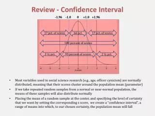
Finding the confidence interval from a list of data 97.8 98.0 98.2 98.2 98.2 98.6 98.8 98.8 99.2 99.4 Finding the confidence interval from the mean and s.d. of a sample Whenever you construct a confidence interval based on t, there are three conditions you must check. Officially, you need a random sample (or random assignment of treatments to units) an approximately normally distributed population or a large enough sample size that the distribution of the sample mean is approximately normal in the case of a survey, the size of the population should be at least ten times the size of the sample. (Listed in detail on pg 569 of textbook)
Quiz Directions • For confidence intervals and significance tests you must show the formula, even if you use your calculator. • No extra time given due to vocabulary • Read directions carefully. • Except for vocabulary answer everything in complete sentences. When you finish work on the homework. 9.1 P#1-5
Warm-upDay 2 of 9.1 Copy the statements and fill in the missing word(s). 1. is the formula for ___________________. 2. When completing a one-proportion z test, you calculate the p-value which informs you whether your p-hat is ____________________ . 3. When writing the hypotheses, the _____________________ is the first one to be considered. The ___________________ is the second one to be considered if the first one is rejected. 4. As sample size increases ____________________ decreases. Word bank: level of confidence, margin of error significance test for a proportion, statistically significant, null hypothesis, alternate hypothesis, test statistic, p-value, critical values, level of significance
b. Using the standard deviation for the sample is not always accurate since it changes based on sample size. Smaller samples will be less accurate and have a larger confidence interval. P2. a. 2.262 b. 2.447 c. 3.106 d. 2.920 e. 2.695 f. 2.637 On calculator a. invT(0.025,9), b. invT(0.025, 6) c. invT(0.005, 11) d. invT(0.05, 2) e. invT(0.005, 43) f. invT(0.005, 81)
P3. a. t* =3.182, t* ∙ The interval is 27 + 19.092, or 7.908 to 46.092 b. t* = 2.306, t* ∙ The interval is 6 + 2.306, or 3.694 to 8.306 c. t* = 2.131, t* The interval is 9 + 25.572, or -16.572
Or use InvT and not the table to get 1.984 invT(.025, 121) = 1.984
9.1 (day 2) confidence interval of the mean Gosset’s model uses the sample standard deviation to approximate the confidence interval using t* (the student’s t) A one-sample t-interval for the mean In 2004, a team of researchers published a study of contaminants in farmed salmon. The study expressed concerns over level of contaminants found. One contaminant found is mirex. In parts per million an average of 0.0913 ppm were found with a std. dev. of 0.0495 ppm in a sample of 150 randomly selected salmon from a particular pond. The distribution of mirex concentration found in the salmon was approximately normal.
Find the 95% confidence interval. Interpret the meaning of the confidence interval in the context of the problem.
T-distribution curve • Notice how the t-distribution curve changes based on the degrees of freedom.
Another example Some students are concerned about safety near an elementary school. Though there is a 15 MPH SCHOOL ZONE sign nearby, most drivers seem to go much faster than that, even when the warning sign flashes. The students randomly select 20 cars passing during the flashing zone times, and recorded the averages. They found that the overall speed during the flashing school zone times for the 20 time periods was 24.6 mph with a std. dev. of 7.24 mph. Find the 90% confidence interval for the average speed of all vehicles passing the school during those hours. A histogram of the data demonstrates the distribution of the average speeds are approximately normal.
9.2 One-sample t-test A recent report on the evening news stated that teens watch an average of 13 hours of TV per week. A teacher at Central High School believes that the students in her school actually watch more than 13 hours per week. She randomly selects 25 students from the school and directs them to record their TV viewing hours for one week. The 25 students reported the following number of hours. Step 1: Check conditions and state test. Step 2: State hypotheses.
n = 25 avg. =____ std. dev. = ___ Step 3: To sketch the t-distribution curve accurately follow the following steps. Homework:9.1 E#2 – 6 and #10 and 12 Bring textbook for textbook review