Analytic hierarchy process
Analytic hierarchy process. Dr. Yan Liu Department of Biomedical, Industrial & Human Factors Engineering Wright State University. Introduction. Conflicting Objectives and Tradeoffs in Decision Problems


Analytic hierarchy process
E N D
Presentation Transcript
Analytic hierarchy process Dr. Yan Liu Department of Biomedical, Industrial & Human Factors Engineering Wright State University
Introduction • Conflicting Objectives and Tradeoffs in Decision Problems • e.g. higher returns vs. lower risks in investment, better performance vs. lower price of computer • Objectives with Incomparable Attribute Scales • e.g. maximize profits vs. minimize impacts on environments • Multi-Attribute Decision Making (MADM) • A study of methods and procedures that handle multiple attributes • Usages • Identify a single most preferred alternative • Rank alternatives • Shortlist a limited number of alternatives for subsequent detailed appraisal • Distinguish acceptable from unacceptable possibilities
Introduction (Cont.) • Types of MADM Techniques • Multiattribute scoring model (in Chapter 4) • Covert attributes to comparable measures • Assign weights to these attributes and then calculate the weighted average of each consequence set as an overall score • Compare alternatives using the overall score • Multi-objective mathematical programming • Tackle complex problems involving a large number of decision variables that are subject to constraints • Analytic hierarchy process (AHP) • Multi-attribute utility theory (MAUT) • …
What is AHP? • A Process that Leads One to (Saaty, 1980) • Structure a problem as a hierarchy or as a system with dependence loops • Elicit judgments that reflect ideas, feelings, and emotions • Represent those judgments with meaningful numbers • Synthesize results • Analyze sensitivity to changes in judgments • AHP also uses a weighted average approach idea, but it uses a method for assigning ratings and weights that is considered more reliable and consistent
Purposes of AHP • To structure complexity in gradual steps from the large to the small, or from the general to the particular, so we can relate them with greater accuracy according to our understanding • To improve our awareness by richer synthesis of our knowledge and intuition; AHP is a learning tool rather than a means to discover the TRUTH
Phases in AHP • Phase 1: Decompose the problem into a hierarchy • Start with an identification of the criteria to be used in evaluating different alternatives, organized in a tree-like hierarchy • Phase 2: Collect input data by pairwise comparisons of criteria at each level of the hierarchy and alternatives • Phase 3: Estimate the relative importance (weights) of criteria and alternatives and check the consistency in the pairwise comparisons • Phase 4: Aggregate the relative weights of criteria and alternatives to obtain a global ranking of each alternative with regards to the goal
Hierarchy GOAL CRITERIA ALTERNATIVES
Maximize Overall Job Satisfaction GOAL Reputation Research Location CRITERIA Growth Benefits Colleagues Job C Job B ALTERNATIVES Job A Hierarchy for a Job Selection Decision
Hierarchy (Cont.) • How to Structure a Hierarchy • Identify the overall objective or goal • Identify criteria to satisfy the goal • Identify, where appropriate, sub-criteria under each criterion • Identify alternatives to be evaluated in terms of the sub-criteria at the lowest level • If the relative importance of the sub-criteria can be assessed and the alternatives can be evaluated in terms of the sub-criteria, the hierarchy is finished • Otherwise, continue inserting levels until it is possible to link levels and set priorities (relative weights) on the elements at each level in terms of the elements at the level above it
More General Goal C3 C1 C2 C21 C22 C31 C32 C33 C11 C13 C12 Sub-criteria at the lowest level More Specific Alternatives Structure of a Hierarchy
Maximize Society’s Overall Benefit Political Factors Health, Safety Environment National Economy Centra- lization Political Cooperative- ness Independ- ence Foreign Trade Capital Resources Cheap Electricity Natural Resources Accidents Long-Term Risks Unavoidable Pollution Coal-fired power plant No big power plants Nuclear power plant Energy Decision in the Parliament of Finland
Hierarchy (Cont.) • How Large Should a Hierarchy Be? • Large enough to capture decision maker’s major concerns • Small enough to remain sensitive to change in what is important
Judgment and Preference • In AHP, we use subjective judgment to express preference and its intensity • e.g. Which of two apples is more red and how strongly more red we perceive it to be • From this preference we derive a scale of relative strength of preference
Pairwise Comparison • Define the relative importance of criteria at each level of the hierarchy and relative importance of alternatives by means of pairwise comparisons Pairwise Comparison Matrix (Wi is the relative weight of ith criterion (alternative))
Pairwise Comparison (Cont.) • Scale for Pairwise Comparisons • 1. Equally preferred • 3. One is moderately preferred over the other • 5. One is strongly preferred over the other • 7. One is very strongly preferred over the other • 9. One is extremely preferred over the other • 2,4,6,8 intermediate values • Reciprocals for inverse comparison
Relative Weights Denote the pairwise comparison matrix and the weight matrix as Then Or λis the eigenvalue of A and W is its corresponding right eigenvector There are n eigenvalues and n corresponding eigenvectors for Anxn
Relative Weights (Cont.) • Consistency • Transitivity • a1>a2 and a2>a3, then a1>a3 • Measurement consistency • aij∙ ajk = aik (aij – the cell at the ith row and jth column of the comparison matrix) • Consistency Index (CI) • A measure of deviation of consistency λmax is the maximum eigenvalue of the pairwise comparison matrix CI = 0 or λmax = n implies perfect consistency CI = 0.1 is the generally accepted threshold value
Or Find Eigenvalues and Eigenvectors , where The solution to the equation is given by You can solve eigenvalue and eigenvector problems in Matlab using the command “[V,E]=eig(A)”, where E is the eigenvalue and V is the corresponding eigenvector
Find Eigenvalues and Eigenvectors Using Matlab Suppose the comparison matrix of three criteria is There is only one non-zero real eigenvalue for the pairwise comparison matrix in AHP eigenvectors λmax =3.0385 Its corresponding eigenvector is (0.9161, 0.3715, 0.1506)T; the three numbers in the eigenvector are proportional to the relative weights of the three criteria eigenvalue
Relative Weights (Cont.) Because relative weights must sum up to 1, we have to normalize the eigenvector by dividing each number in it by the sum of all numbers e.g. In the previous example, the eigenvector is (0.9161, 0.3715, 0.1506)T The normalized eigenvector is =(0.64, 0.26, 0.10)T Relative weights for the three criteria CI=(λmax-n)/(n-1) = (3.0385-3) /(3-1) = 0.0193
Satisfaction With School GOAL Friends Vocational Training Music Classes Learning School Life College Preparation CRITERIA School A School C ALTERNATIVES School B School Selection Example
Pairwise Comparison Matrix of Six Criteria (L,F,SL,VT,CP, and MC denote Learning, Friends, School Life, Vocational Training, College Preparation, and Music Classes, respectively)
Using Matlab, we can get λmax =6.2397, and its corresponding eigenvector is ( -0.6773, -0.2198, -0.1908, -0.5780, -0.3212, 0.1389)T The normalized eigenvector is (0.32, 0.10, 0.09, 0.27, 0.15, 0.07)T CI =( 6.2397 – 6) / (6 – 1) = 0.048 < 0.1
Weight 0.16 0.59 0.25 Pairwise Comparison Matrix of Three Alternative Schools With Respect to Learning λmax=3.0536, , and the normalized eigenvector is (0.16, 0.59, 0.25)T CI =( 3.0536 – 3) / (3 – 1) = 0.027
Weight 0.33 0.33 0.33 Pairwise Comparison Matrix of Three Alternative Schools With Respect to Friends λmax=3, and the normalized eigenvector is (1/3, 1/3, 1/3)T CI =( 3 – 3) / (3 – 1) = 0
Weight 0.46 0.09 0.46 Pairwise Comparison Matrix of Three Alternative Schools With Respect to School Life λmax=3, and the normalized eigenvector is (0.46, 0.09, 0.46)T CI =( 3 – 3) / (3 – 1) = 0
Weight 0.77 0.05 0.17 Pairwise Comparison Matrix of Three Alternative Schools With Respect to Vocational Training λmax=3.2085, and the normalized eigenvector is (0.77, 0.05, 0.17)T CI =( 3.2085 – 3) / (3 – 1) = 0.104
Weight 0.25 0.50 0.25 Pairwise Comparison Matrix of Three Alternative Schools With Respect to College Preparation λmax=3, and the normalized eigenvector is (0.25, 0.50, 0.25)T CI =( 3 – 3) / (3 – 1) = 0
Weight 0.69 0.09 0.22 Pairwise Comparison Matrix of Three Alternative Schools With Respect to Music Classes λmax=3.053, and the normalized eigenvector is (0.69, 0.09, 0.22)T CI =( 3.0536 – 3) / (3 – 1) = 0.027
Relative Weights (Cont.) • Other than computing the eigenvector of a pairwise comparison matrix to find the weights of compared criteria or alternatives, we can also approximate the weight by: • First, normalizing each column in the comparison matrix • Then, calculating the average of each row in the normalized matrix as the estimate of the relative weight for its corresponding criterion or alternative
T2 Tn CM2= CM1= CMn= Tn T2 Tn T2 … Total Tn= T2= T1= CI ≈ Consistency Measure Approximated Weight T1 T1 … … T1
School Selection Example (Cont.) Sum 3.17 10.50 12.50 3.87 7.00 14.00 Pairwise Comparison Matrix of Six Criterion
Eigenvector Weight Approximated Weight 0.32 0.32 0.10 0.10 0.09 0.09 0.27 0.27 0.15 0.15 0.07 0.07 Normalized Pairwise Comparison Matrix of Six Criteria
CM1= Consistency Measure Approximated Weight 6.22 0.32 6.5 0.10 6.29 0.09 6.30 0.27 6.31 0.15 5.86 0.07 CM2= Likewise, we can calculate CM3, CM4, CM5, and CM6 CI =0.048 from eigenvalue CI ≈
Approximated Weight 0.16 0.59 Sum 6 1.67 4.5 0.25 Pairwise Comparison Matrix of Three Alternative Schools With Respect to Learning Normalized Pairwise Comparison Matrix of Three Alternative Schools With Respect to Learning
Consistency Measure Approximated Weight 3.01 0.16 3.08 0.59 3.07 0.25 CM1= CM2= CM3= CI ≈
Composition and Synthesis • Combine the relative importance of criteria and alternatives to obtain a global ranking of each alternative with regards to the goal Criteria Cj (j=1,2,…,n) and their corresponding weights Composite impact OA1 = wC1wA1C1+wC2wA1C2+…+wCnwA1Cn OA2 = wC1wA2C1+wC2wA2C2+…+wCnwA2Cn … OAm = wC1wAmC1+wC2wAmC2+…+wCnwCnAm Weights of alternatives Ai (i=1,2,…,m) w.r.t. criteria Cj (j=1,2,…,n)
OA=0.32*0.16+0.10*0.33+0.09*0.45+0.27*0.77+0.15*0.25+0.07*0.69 = 0.42 OB=0.32*0.59+0.10*0.33+0.09*0.09+0.27*0.05+0.15*0.5+0.07*0.09 = 0.33 OC=0.32*0.25+0.10*0.33+0.09*0.46+0.27*0.17+0.15*0.25+0.07*0.22 = 0.25 In conclusion, school A seems to be the best, and C seems to be the worst
Summary of AHP • Applications of AHP • e.g. resource allocation , conflict resolution, prediction, planning, etc. • Advantages • Decision hierarchy and pairwise comparisons make the AHP process easy to comprehend • The use of a subjective scale, such as “strongly preferred”, rather than a quantitative scale is particularly useful when it is difficult to formalize some criteria (attributes) quantitatively • It is usually much easier to compare two items at a time than to compare many items all at once • Disadvantages • The decision hierarchy in AHP assumes independence among criteria, which is not always appropriate • The subjective scale is subject to human errors and biases • The number of pairwise comparisons becomes quite extensive when the number of attributes and alternatives is large