Download
1 / 19
250 likes | 789 Vues
Correlation Analysis. Correlation Analysis: Introduction. Management questions frequently revolve around the study of relationships between two or more variables. Thus a relational hypothesis is necessary. Various Objectives are served with correlation analysis.

E N D
Correlation Analysis: Introduction • Management questions frequently revolve around the study of relationships between two or more variables. Thus a relational hypothesis is necessary. • Various Objectives are served with correlation analysis. • The strength, direction, shape and other features of the relationship may be discovered. • With correlation, one calculates an index to measure the nature of the relationship between variables
Bivariate Correlation Analysis (BCA) • The Pearson (product moment) correlation coefficient varies over a range of +1 through to – 1. • The designation r symbolizes the coefficient’s estimate of linear association based on sampling data. • The coefficient p represents the population correlation.
BCA contd. • Correlation coefficient reveal the magnitude and direction of relationships. • The magnitude is the degree to which variables move in unison or opposition. • The size of a correlation of +.40 is the same as one of -.40. • The sign says nothing about size. • The degree of correlation is modest.
BCA contd. • Direction tells us whether two variables move in the same direction, opposite direction. • When variables move in the same direction, the two variables have a positive relationship: • As one increases, the other also increases • Family income, e.g., is positively related to household food expenditure. • As income increases, food expenditures increase.
BCA contd. • Some variables move in the opposite direction, e.g., the prices of products/ services and their demand. These variables are inversely related. • The absence of a relationship is expressed by a coefficient of approximately zero.
Scatterplots for Exploring Relationships • Scattoerplot are essential for understanding the relationships between variables. • They provide a means for visual inspection of data that a list of values for two variables cannot. • Both the direction and the shape of a relationship are conveyed in a plot. • The magnitude of the relationship can also be seen.
Correlation Matrix • The correlation is one of the most common and most useful statistics. • A correlation is a single number that describes the degree of relationship between two variables.
Correlation Example • Let's assume that we want to look at the relationship between two variables, height (in inches) and self esteem. • Our hypothesis is that height affects one's self esteem (The direction of causality is not taken into account, i.e., it's not likely that self esteem causes one’s height). • Data on the age and height of twenty individuals are collected. We know that the average height differs for males and females, so, to keep this example simple, the example uses males only. • Height is measured in inches. Self esteem is measured based on the average of 10, 1-to-5, rating items (where higher scores mean higher self esteem). Here's the data for the 20 cases: Table 1 in WORD Format
Example contd. • We use the symbol r to stand for the correlation. The value of r will always be between -1.0 and +1.0. if the correlation is negative, we have a negative relationship; if it's positive, the relationship is positive. • N = 20 • ∑XY = 4937.6 • ∑X = 1308 • ∑Y = 75.1 • ∑X2 = 85912 • ∑Y2 = 285.45
Example contd. • Plugging these values into the formula given above, we get the value of r: r = 0.73 • So, the correlation for our twenty cases (.73) is shows a fairly strong positive relationship. • It seems that there is a relationship between height and self esteem, at least in this made up data!
Testing the Significance of a Correlation • After having computed a correlation, we can determine the probability that the observed correlation occurred by chance. • This can be done by conducting a significance test. • Most often we are interested in determining the probability that the correlation is a real one and not a chance occurrence. • In this case, we are testing the mutually exclusive hypotheses:
Testing the Significance • Null Hypothesis: r = 0 • Alternative Hypothesis: r <> 0 • The easiest way to test this hypothesis is to find a statistics book that has a table of critical values of r. • Most introductory statistics texts would have a table like this. As in all hypotheses testing, we need to first, determine thesignificance level.
Testing the Significance contd. • Here, we will use the common significance level of alpha = .05. • This means that we are conducting a test where the odds that the correlation is a chance occurrence are no more than 5 out of 100. • Second, before we look up the critical value in a table we also have to compute the degrees of freedom (df). • The df is simply equal to N-2 or, in this example, is 20-2 = 18.
Testing the Significance contd. • Finally, we have to decide whether we are doing a one-tailed or two-tailed test. • In this example, since we have no strong prior theory to suggest whether the relationship between height and self esteem would be positive or negative, we will opt for the two-tailed test.
Testing the Significance contd. • With the following three pieces of information • the significance level (alpha = .05)), • degrees of freedom (df = 18), and • type of test (two-tailed) • we can now test the significance of the correlation we have found. • The critical value in the statistics book is .4438.
Testing the Significance contd. • This means that if the computed value of correlation is greater than .4438 or less than -.4438 (remember, this is a two-tailed test), we can conclude that the odds are less than 5 out of 100 that this is a chance occurrence. • Since our computed correlation 0f 0.73 is quite higher, we conclude that it is not a chance finding and that the correlation is "statistically significant" (given the parameters of the test). We can reject the null hypothesis and accept the alternative.