Download
1 / 31
330 likes | 546 Vues
INTERFEROMETRIC RADIOMETRY MEASUREMENT CONCEPT: THE VISIBILITY EQUATION. I. Corbella, F. Torres, N. Duffo, M. Martín-Neira. Interferometric Radiometry. Technique to enhance spatial resolution without large bulk antennas.

E N D
INTERFEROMETRIC RADIOMETRY MEASUREMENT CONCEPT: THE VISIBILITYEQUATION I. Corbella, F. Torres, N. Duffo, M. Martín-Neira
Interferometric Radiometry • Technique to enhance spatial resolution without large bulk antennas. • Based on cross-correlating signals collected by pairs of ”small” antennas (baselines). • Image obtained by a Fourier technique from correlation measurements. No scanning needed. • Examples: • Precedent: Michelson (end of 19th century). Astronomical observations at optical wavelengths. • Radioastronomy: Very Large Array (1980). 27 dish antennas, 21 km arm length Y-shape. Various frequencies. • Earth Observation: SMOS (2009). 69 antennas, 4m arm length Y-shape. L-band. IGARSS 11. Vancouver. Canada
Interferometry: Fringes vd distant point source 2A2 z Δr=d cos α0 A2 α0 x d b1 b2 Δℓ Δℓ/λ Δr/λ Quadratic detector Total power Cross-correlation IGARSS 11. Vancouver. Canada
vd uΔξ 2I 0 0.5 0.75 I 1 Δℓ/λ Δr/λ Fringe Visibility distant small source with constant intensity I z Δξ Δr=d cos α0 α0 x d b1 b2 Δℓ ξ0=cos α0 u=d/λ Δr/λ=uξ0 vd Michelson’s “Fringe Visibility”: Cross-correlation for Δℓ=0: IGARSS 11. Vancouver. Canada
Complex Visibility Definition • Michelson’s “fringe visibility” is the amplitude of the complex visibility |V(u)|=I·|sinc uΔξ| normalized to the total intensity of the source. • The cross correlation between both signals for Δℓ=0 is the real part of the complex visibility <b1b2>=Re[V(u)]. The imaginary part is obtained by adding a 90º phase shift (quarter wavelength) to one of the signals. • The complex visibility is the Fourier Transform of the Intensity distribution expressed as a function of the director cosine ξ: V(u)=F[I(ξ)] z I(ξ) V(u) I0Δξ=I Δξ ξ=cos α I0 Δξ α ξ0 ξ u x d b1 b2 u=d/λ IGARSS 11. Vancouver. Canada
Interferometric radiometres Use Brightness Temperature (TB) instead of intensity (I): 1-D y u x • The spatial resolution is achieved • by synthesized beam in ξ • by antenna pattern in η d y 2-D u v d x • The spatial resolution is achieved by synthesized beam in both dimensions (ξ and η). • Different options for geometry: • Y-shape, Rectangular, T-shape, Circle, Others d IGARSS 11. Vancouver. Canada
Spatial resolution: Synthetic beam Direct equation Fourier inversion Only limited values of (u,v) are available: The measured visibility function is necessarily windowed. Retrieved brightness temperature Convolution integral • Array Factor: Inverse Fourier transform of the window • It is the “synthetic beam”. It sets the spatial resolution • Its width depends on the maximum (u,v) values (antenna maximum spacing) IGARSS 11. Vancouver. Canada
Comparison with real apertures Rectangular u-v coverage and no window v vM A=Δxmax, B=Δymax: Maximum distance between antennas in each direction u -vM -uM uM Physical aperture with uniform fields y x B 0.60 (for small angles around boresight) 0.88 A IGARSS 11. Vancouver. Canada
Examples of Synthetic beam Y-shape instrument (19 antennas per arm) Rectangular window Blackmann window = 1.73 deg = 2.46 deg IGARSS 11. Vancouver. Canada
Microwave Radiometry formulation • Power spectral density: • Antenna temperature Extended source of thermal radiation b1 r1 r2 TB(θ,) • Cross-Power spectral density: • Visibility b2 (units: Kelvin) (complex valued) Antenna power pattern phase difference Antenna field patterns IGARSS 11. Vancouver. Canada
The anechoic chamber paradox anechoic chamber at constant temperature • Power spectral density: Antenna temperature T b1 TA=T (OK!) T • Cross Power spectral density: Visibility b2 T V12 is apparently non-zero and antenna dependent But V12 should be zero (Bosma Theorem) Experiments confirm that V12=0 IGARSS 11. Vancouver. Canada
The “–Tr” term The solution is found when all noise contributors are taken into account. a1 T b1 a2 Tr b2 Cross power spectral density for total output waves: Tr Consistent with Bosma theorem: • Tr: equivalent temperature of noise produced by the receivers and entering the antennas. This noise is coupled from one antenna to the other. • If the receivers have input isolators, Tr is their physical temperature. IGARSS 11. Vancouver. Canada
Empty chamber visibility Result from IVT at ESA’s Maxwell Chamber IGARSS 11. Vancouver. Canada
Cold Sky Visibility Sky Sky Arm A Arm B Chamber Chamber Arm C Sky Blue: SMOS at ESA’s Maxwell Chamber Red: SMOS on flight during external calibration Chamber IGARSS 11. Vancouver. Canada
Limited bandwidth and time correlation Average power Bandwidth: B1 Gain: G1 bs1 b1 Receiver 1 TA: Antenna temperature (K) Centre frequency: f0 bs2 TR: Receiver noise temperature (K) Receiver 2 b2 Complex correlation Bandwidth: B2 Gain: G2 b1,2(t): Analytic signals V12: Visibility (K) Fringe washing function IGARSS 11. Vancouver. Canada
Director cosines and antenna spacing At large distances (R>>d1) distant source point z R θ Antenna location at coordinates (x1,y1,z1) r1 d1 y Director cosines x For two close antennas in the x-y plane: Phase difference: Antenna normalized spacing IGARSS 11. Vancouver. Canada
The visibility equation Physical temperature of receivers Tr=(Trk+Trj)/2 Antenna relative spacing: Decorrelation time: Notes: * ukj and vkj are defined in terms of the wavelength at the centre frequency. * The visibility has hermiticity property IGARSS 11. Vancouver. Canada
The zero baseline • V(0,0) is equal to the difference between the antenna temperature and the receivers’ physical temperature. • It is redundant of order equal to number of receivers. • At least one antenna temperature must be measured. • In SMOS, two methods have been considered: • Three dedicated noise-injection radiometers (NIR) • All receivers operating as total power radiometers. • The selected baseline method is the first one (NIR) putting u=v=0 V(0,0)=TA-Tr IGARSS 11. Vancouver. Canada
Polarimetric brightness temperatures Spectral power density: Observation point ΔΩ if Thermal radiation (p,q): orthogonal polarization basis (linear, circular, …) Brightness temperature at p polarisation: Brightness temperature at q polarisation: Complex Brightness temperature at p-q polarisations: Relation with Stokes parameters: IGARSS 11. Vancouver. Canada
Polarimetric interferometric radiometer Visibility at pp polarization Visibility at qq polarization Visibility at pq polarization Visibility at qp polarization IGARSS 11. Vancouver. Canada
Image Reconstruction Visibility: For any pair of antennas k,j (k≠j) (hermiticity) Physical temperature of receivers: Trkj=(Trk+Trj)/2 Antenna relative spacing: Antenna Temperature: For any single antenna k IGARSS 11. Vancouver. Canada
The Flat-Target response Definition The visibility of a completely unpolarised target having equal brightness temperature in any direction (“flat target”) is: Measurement It can be measured by pointing the instrument to a known flat target as the cold sky (galactic pole). Estimation It can also be estimated (computed) from antenna patterns and fringe washing functions measurements. For large antenna separation, FTR≈0 IGARSS 11. Vancouver. Canada
Image reconstruction consists of solving for T(ξ,η) in the following equation where (zero outside) and V and T depend of the approach chosen: T(ξ,η) is only function of (ξ,η) Approach #1 #2 #3 IGARSS 11. Vancouver. Canada
pair (k,j): u=(xj-xk)/λ0 v=(yj-yk)/λ0 Hexagonal sampling (MIRAS) Na: Total number of antennas • Number of antenna pairs: Na(Na-1)/2 NEL : Number of antennas in each arm. An antenna in the centre is considered. • Number of unique (u-v) points: 3[NEL(NEL+1)] • Number of points in the “star”: 6[NEL(NEL+1)]+1 Example: NEL=6; d=0.875 13 u,v points Antenna Positions and numbering Hermitic values 3[NEL(NEL+1)]=126 u v 8 1 7 14 NEL=6 Na=3NEL+1=19 Principal values 253 total points 3[NEL(NEL+1)]=126 19 IGARSS 11. Vancouver. Canada
Aliasing Discrete sampling produces spatial periodicity: Aliases Visibility: (u-v) domain Brightness temperature: (ξ-η) domain Alias-free Field Of View (FOV): Zone of non-overlapping unit circle aliases Unit circle IGARSS 11. Vancouver. Canada
Strict and extended alias-free field of view Unit Circle Earth Contour Antenna Boresight Unit Circle aliases Earth aliases Alias-Free Field of View Extended Alias-Free Field of view Zone of non-overlapping unit circles Zone of non-overlapping Earth contours IGARSS 11. Vancouver. Canada
Projection to ground coordinates Boresight Nadir Swath: 525 km IGARSS 11. Vancouver. Canada
Geo-location • The regular grid in xi-eta is mapped into irregular grid in longitude-latitude Irregular grid in lat-lon Regular grid in director cosines IGARSS 11. Vancouver. Canada
Full polarimetric SMOS snapshot North-west of Australia IGARSS 11. Vancouver. Canada
SMOS sky image IGARSS 11. Vancouver. Canada
Conclusions • Interferometric radiometry has a long heritage that goes back to the 19th century. SMOS has demonstrated its feasibility for Earth Observation from space. • The complete visibility equation for a microwave interferometer must include the effect of antenna cross coupling and receivers finite bandwidth. • Image reconstruction is based on Fourier inversion. Improved performance is achieved by using the flat target response. • Aliasing induces a complex field of view. In SMOS two zones with different data quality exist: Alias-free and extended alias-free. • Spatial resolution, sensitivity, incidence angle and rotation angle have significant variations inside the Field of view. IGARSS 11. Vancouver. Canada