Download
1 / 10
110 likes | 375 Vues
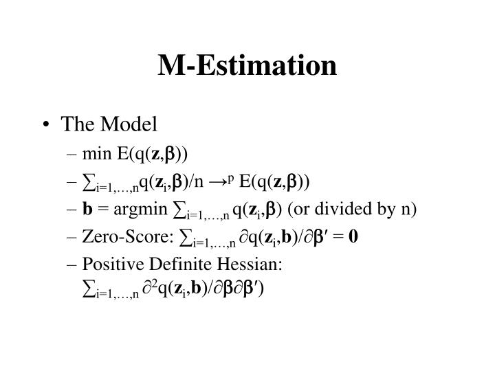
M-Estimation. The Model min E(q( z , b )) ∑ i=1,…,n q( z i , b )/n → p E(q( z , b )) b = argmin ∑ i=1,…,n q( z i , b ) (or divided by n) Zero-Score: ∑ i=1,…,n q( z i , b )/ b ′ = 0 Positive Definite Hessian: ∑ i=1,…,n 2 q( z i , b )/ b b ′ ). NLS, ML as M-Estimation.

E N D
M-Estimation • The Model • min E(q(z,b)) • ∑i=1,…,nq(zi,b)/n →p E(q(z,b)) • b = argmin ∑i=1,…,n q(zi,b) (or divided by n) • Zero-Score: ∑i=1,…,n q(zi,b)/b′ = 0 • Positive Definite Hessian: ∑i=1,…,n 2q(zi,b)/bb′)
NLS, ML as M-Estimation • Nonlinear Least Squares • y = f(x,b) + e, z =[y,x] • S(β) = ε′ε = ∑i=1,…,n (yi-f(xi,b))2 • q(yi,xi,b) = (yi-f(xi,b))2 • b = argmin S(β) • Maximum Log-Likelihood • ll(β) = ∑i=1,…,n ln pdf(yi,xi,b) • q(yi,xi,b) = ln pdf(yi,xi,b) • b = argmin -ll(β)
The Score Vector • s(z,b) = q(z,b)/b′ • E(s(z,b)) = E(q(z,b)/b′) = 0 • ∑i=1,…,n s(zi,b)/n →p E(s(z,b)) = 0 • V = Var(s(z,b)) = E(s(z,b)s(z,b)′) = E((q(z,b)/b′) (q(z,b)/b) ) • ∑i=1,…,n [s(zi,b)s(zi,b)′]/n →P Var(s(z,b)) • ∑i=1,…,n s(zi,b)/n →dN(0,V)
The Hessian Matrix • H(z,b) = E(s(z,b)/b) = E(2q(z,b)/bb′) • ∑i=1,…,n [s(zi,b)/b]/n →pH(z,b) • Information Matrix Equality does not necessary hold in general: - H ≠ V • More general than NLS and ML
The Asymptotic Theory • n(b-b) = {∑i=1,…,n [s(zi,b)/b]/n}-1[∑i=1,…,n s(zi,b)/n] • n(b-b) →dN(0,H-1VH-1) • V = E(s(z,b)s(z,b)′) = E[(q(z,b)/b)′(q(z,b)/b)] • H = E(s(z,b)/b) = E(2q(z,b)/bb′) • ∑i=1,…,n [s(zi,b)s(zi,b)′]/n →pV • ∑i=1,…,n [s(zi,b)/b]/n →pH
Asymptotic Normality • b →pb • b ~aN(b,Var(b)) • Var(b) = H-1VH-1 • H and V are evaluated at b: • H= ∑i=1,…,n [2q(zi,b)/bb′] • V = ∑i=1,…,n [q(zi,b)/b][q(zi,b)/b′]
Application • Heteroscedastity Autocorrelation Consistent Variance-Covariance Matrix • Non-spherical disturbances in NLS • Quasi Maximum Likelihood (QML) • Misspecified density assumption in ML • Information Equality may not hold
Example • Nonlinear CES Production Functionln(Q) = b1 + b4 ln[b2Lb3+(1-b2)Kb3] + e • NLS (homoscedasticy) • NLS (robust covariances) • ML (normal density) • QML (misspecified normality)
Example Nonlinear CES Production Function
Example • Nonlinear CES Production Function