Download
1 / 72
790 likes | 950 Vues
NMR Spectroscopy. A short introduction. How it all began. How it all began. Bloch, Felix, (1905–83), Swiss-American physicist and Nobel laureate, born in Zürich, Switzerland, and educated at the Federal Institute of Technology there

E N D
NMR Spectroscopy A short introduction
How it all began.... Bloch, Felix, (1905–83), Swiss-American physicist and Nobel laureate, born in Zürich, Switzerland, and educated at the Federal Institute of Technology there and in Germany at the University of Leipzig. He left Germany in 1933 and a year later he joined the faculty of Stanford University in California, where he taught until his retirement in 1971. Bloch’s doctoral dissertation (1928) is recognized as the basis of the modern theory of solids. He also made significant contributions to theoretical physics, particularly to the fields of superconductivity and magnetism. During World War II he worked on the Manhattan Project (the first atomic bomb) and on war-related counter-radar research. In 1946, Bloch became known for his method of determining the magnetic moment (a measure of magnetic strength) of the neutron and the development of the technique called nuclear magnetic resonance. He shared the 1952 Nobel Prize in physics with the American physicist Edward M. Purcell, who had independently discovered, in a different way, nuclear magnetic resonance at about the same time.
..and we need a magnetic field 400MHz = 9.395 T (tesla) = 9.395*104 G (gauss)
Quantum spin number 0 nucleus is magnetically active • e.g. 1H, 13C, 15N, 19F, 31P (I = 1/2) • They will be observed at different (well separated ) frequencies. • We normally just detect one nucleus at a time! • 15N 13C 31P 19F 1H Basics of NMR Spectroscopy
p Nuclear Spins The nucleus has a spin (rotation) The angular momentump is a vector parallel to the axis of rotation The magnitude of the angular momentum is given by the spin quantum numberI: p = h/2p * I(I+1)
p Nuclear Spins A circulating current creates a ring current The ring current creates a dipolar magnetic moment: m = g p g: gyromagnetic ratio The gyromagnetic ratio is a constant for each nucleus, describing its magnetic properties
m p Nuclear Spins The magnetic moment m is a vector parallel to the angular momentum p
N N N N N S S S S S Nuclear Spins Outside a magnetic field the nuclear spins have no orientation
N S S S S S S N N N N N Bo Nuclear Spins Inside a magnetic field the nuclear spins will be aligned along the magnetic field axis The picture shown here is not really correct: quantum mechanics allows only discrete orientations The number of possible orientations is given by the spin quantum number I
N -Em / kT -Em / kT e e N N N S S S S S S S S S N N N N N Bo Nuclear Spins Not all nuclei align parallel The number of nuclei with parallel and anti-parallel orientation is described by Boltzmann‘s law: Nm = No m
N -Em / kT -Em / kT e e N N N S S S S S S S S S N N N N N Bo Nuclear Spins Nm : number of spins in state m No : total number of spins Em : energy of state m k : Boltzmann constant T : temperature Nm = No m
N N N N S S S S S S S S S N N N N N Bo Nuclear Spins How many spins have parallel and anti-parallel orientation? N+ - N- = NoDE /2kT Assuming: Bo = 1 Tesla (43MHz) No = 2‘000‘000 N+ = 1‘000‘001 N- = 999‘999
m=-1/2 N N N N DE = g h Bo S S S S S S S S S N N N N N m=1/2 E Bo Bo Nuclear Spins The energy levels are called Zeeman levels
In a magnetic field, the Zeeman levels are splitted according to: type of the nucleus strength of the magnetic field 1H has a higher frequency than 13C at the same field strength 1H is more sensitive than 13C at the same field strength 1Hsplitting E 13Csplitting field What do we Observe ? (1)
What do we Observe ? (2) Levels with different energies have different populations p: Equilibrium population We use rf pulses (MHz) in order to perturb the system : Perturbed population We observe populations going back to equilibrium: B A E A D ¹ p 0 E B D = p 0
m=-1/2 m=+1/2 E Nuclear Spins: macroscopic magnetisation
From Microscopic to Macroscopic B 0 z M y x rf pulse 90° flip angle z M = magnetisation vector B0 = static magnetic field y M x
Macroscopic Signal z y M Magnetisation precesses at a frequency given by : the type of nucleus the electronic environment in the molecule Magnetisationrelaxes towards equilibrium The detected signal, the FID ("Free Induction Decay") shows : frequency of precession damping due to relaxation x z y M x time T =1/
Macroscopic Signal z wI y M x z • Resonance Condition of NMR Spectroscopy: • wI = gI Bo • wI :Larmor frequency • gI :gyromagnetic ratio • Bo:magnetic field
Signal Processing FT time Frequency or chemical shift via the Fourier Transform To understand the signal, we go from the time domain signal, the FID, to the frequency domain signal, the spectrum
Summary • Nuclei have a spin which creates a magnetic moment. • Due to the magnetic moment the nuclei will orientate in the magnetic field and thus create a net-magnetisation, called ‚macroscopic‘ magnetisation. • The orientation of the macroscopic magnetisation will be disturbed by a RF pulse, thus creating a magnetisation vector in the x,y frame. • The magnetisation rotates in the x,y, frame and induces a voltage in a receiver coil. • The induced signal is processed by Fourier transformation
wo z z M M wo y y’ x’ x Laboratory and Rotating Frame • Rotating Frame: • The x,y, frame is rotating with the Larmor frequency wo • The magnetisation is seen at a fix position • Laboratory Frame: • The x,y, frame is fix with respect to an external observer. • The magnitization is seen rotating with the Larmor frequency wo
z B1 y x The RF pulse Laboratory Frame 1. A coil is installed with its long axis oriented along the x axis. 2. This ‚transmitter coil‘ is feeded with an alternating current 3. A magnetic field oscillating linearly along the x axis
B1 time The RF pulse 1. The oscillating B1 field can be considered as being composed of two opposite rotating components. 2. These two components are located in the x,y frame
z B1 y x B1ac B1c B1ac:B1 component, rotates anti clockwise B1c:B1 component, rotates clockwise The RF pulse Laboratory Frame 1. The oscillation frequency of B1candB1acis: = 2p n 2. The oscillating frequency will be set equal to the frequency of the rotating frame: = wo 3. One component, B1c or B1ac then will be static with respect to the rotating frame
z y x B1c static The RF pulse Rotating Frame 1. The macroscopic magnetization Mz will rotate along the static component of the B1 field. 2. Any macroscopic magnetization aligned exactly with the static component of the B1 field will not move. a Mz
z Rotating Frame a Mz y B1c static x tp time RF The RF pulse 1. The rotation angle a depends on how long the field B1 is applied 2. Definitions: a : pulse or flip angle tp: time of B1 switched on tp(90) time required for a 90o rotation 90o pulse: RF flips a macroscopic magnetization by 90o
W +1/tp W -1/tp frequency tp W time RF The RF pulse 1. The excitation bandwidth is defined by the length of the 90o pulse 2. The excitation profile is described by a SINC-function 2. A short duration for the 90o pulse is required for a uniform excitation over the entire spectral range Excitation profile = sinc(0.5(w-W)tp)
z M Mz a y My x The RF pulse 1. The intensity and phase of the NMR signal is given by the size and phase of the Mx,y magnetization 2. The magnetization vector can be described by the two projections to the z- and the x-/y-axis 3. The magnetization Mz does not create a NMR signal
The NMR experiment: what do we need? 1. The magnet 2. The probe head 3. Generation of RF pulses for excitation 4. Preamplification of received signals 5. Digital processing of analog NMR signal
The NMR experiment: what do we need? • 1. The magnet: • Requires control of field homogeneity SHIM • Requires stabilisation of main field LOCK • SHIM: • additional coils with special field distribution, • e.g. Z, Z2, Z3, X, Y, X3.... • We have cryo shims and room temperature shims • LOCK • 1.contineously determines frequency of 2H signal of the • solvent (deuterated solvents) • 2. add a small extra field to the main field of the magnet • to keep the overall field constant • 3. 2H signal also used for shimming
Basics of shims Shims are used to compensate the magnetic field inhomogeneity in the sample area Compensation is done by creating a magnetic field profile which has: • opposite sign compared to the inhomogeneity • same absolute intensity as inhomogeneity Compensation requires a shim system to create the compensation field
Z1 Z2 Z3 Z Z Z Z Z Z4 Z5 Basics of shims Shim field functional forms of some on-axis shims The Z axis is the axis of the magnet and the NMR sample tube
DBo Z Z DBShim DB0 Z Z1 Z2 Z Z Basics of shims Example: an inhomogeneity which would require the shim functions Z1 and Z2 to be adjusted The magnet‘s field before correction correction field of the shim coil superposition of magnet‘s field and the correction field
The NMR experiment: what do we need? • 1. The magnet: • Requires control of field homogeneity SHIM • Requires stabilisation of main field LOCK • SHIM: • additional coils with special field distribution, • e.g. Z, Z2, Z3, X, Y, X3.... • We have cryo shims and room temperature shims • LOCK • 1.contineously determines frequency of 2H signal of the • solvent (deuterated solvents) • 2. add a small extra field to the main field of the magnet • to keep the overall field constant • 3. 2H signal also used for shimming
The resonance condition of NMR: w=g Bobut: Bo is not stable w=g (Bo+Ho)(Bo+Ho) = const. Shim system Regulator Ho amplitude, frequency Probe Transmitter 2H Receiver 2H The lock: details The lock channel can be understood as a ‚completely indepenant spectrometer within the spectrometer‘:
F=0o absorption: signal F=90o dispersion: The lock: lock phase The lock receiver has two quadrature channels:
Intensity The lock: field homogenisation The absorption signal is used for field homogenisation The signal intensity is a measure for the field homogeneity: sharp signal, high lock level broad signal, low lock level
The lock: field stabilisation The dispersion signal is used for field stabilisation The position of the zero-crossing of the signal is permanently checked Determination of the zero-crossing frequency is more sensitive than determination of the frequency at maximum peak position
wo(2H) wo(2H) The lock: field stabilisation
The lock: lock phase If the lock phase is not adjusted correctly, absorption and dispersion signals will be mixed Non-pure phases will result in: • imperfect field homogenisation (shimming) • imperfect field homogenisation • field shifts during experiment using pulsed field gradients
The lock: lock phase and GRASP WATERGATE experiment: top: correct lock phase bottom: lock phase wrong by 30o
The lock: regulation parameters Regulation parameters: Loop Gain: how strong to react on field disturbance Loop Time: how fast to react „ „ „ Loop Filter:smoothing the lock signal to remove noise, low pass filter Wrong settings will result in: • instable signal position: suppression artifacts (NOE-difference,...) • noise around the signal Use xau loopadj for adjusting the loop parameters
The lock: further parameters Lock power: • 2H transmitter output power • Due to different relaxation behavior of 2H for individual solvents, the lock power has to be adjusted for each solvent • Too high lock power will result in an unstable lock signal Lock gain: • receiver gain of the lock channel • Gain too low: field homogenisation not optimum • Gain too high:receiver is not linear, field homogenisation not optimum, spikes around NMR signals
The NMR experiment: what do we need? • 2. The probe head: • Mainly is an antenna • typically 3 RF channels: • 2H: for the LOCK and shimming • 1H: for 1H-NMR and 1H-decoupling • X: e.g. 13C, for 13C-NMR and 13C decoupling • The susceptibility of the coil material is crucial for • best line shape of the NMR signal
The NMR experiment: the probe Helmholtz coils are mainly used for high resolution applications. Example of a Helmholtz coil design
The NMR experiment: what do we need? Sample location in the probehead
The probe Pulse power: • Do not apply pulses at a power higher than specified for the probe • During endtest of the spectrometer the shortest possible pulses are calibrated. For pulse sequences those power levels might be too high, e.g. for 1H trim pulses in HSQC • Carefully check the tuning and matching of the transmitter and decoupler channel