Download
1 / 28
280 likes | 373 Vues
SZ effects by using high-resolution simulations. Lauro Moscardini Dipartimento di Astronomia Università di Bologna, Italy lauro.moscardini@unibo.it. Works in collaboration with: S. Borgani, A. Diaferio, K. Dolag, G. Murante, M. Roncarelli, V. Springel, G. Tormen, L. Tornatore, P. Tozzi.

E N D
SZ effects by using high-resolution simulations Lauro Moscardini Dipartimento di Astronomia Università di Bologna, Italy lauro.moscardini@unibo.it Works in collaboration with:S. Borgani,A. Diaferio, K. Dolag,G. Murante,M. Roncarelli,V. Springel, G. Tormen, L. Tornatore, P. Tozzi. Mainly based onDiaferio et al. 2005, MNRAS, 356, 1477; Roncarelli et al. 2005, in preparation; Bonaldi et al. 2005, in preparation Orsay, Paris, 7-8th april 2005
A Tree+SPH high-res. Simulation of the cosmic web KP Collaboration: S. Borgani, A. Diaferio, K. Dolag, L. Moscardini, G. Murante, V. Springel, G. Tormen, L.Tornatore, P.Tozzi Co-workers: M. Arnaboldi, L.M. Cheng, S. Ettori, O. Gerhard, E. Rasia, M. Roncarelli, plus other students Code:Tree + SPHGADGET (Springel et al. 2001, 2002) www.MPA-Garching.MPG.DE/gadget Radiative cool.+UV backgr. Multiphase model for star-formation and model galactic winds. CDM cosmology: m= 1-0.3 , bar0.02h-2 , h=0.7 , 8=0.8 L = 192 h-1 Mpc ; Ngas=NDM= 4803 Pl= 7.5 h-1 kpc ; mgas= 6.9 108 h-1M⊙ 40,000 CPU hours and 100 Gb RAM, using 64 processors of IBM-SP4 in CINECA (INAF grant); about 1.2 Tb of data produced.
400 clusters with > 104particles. X-ray cluster scaling properties and nature of their scatter. Contribution of diffuse gas to the soft X-ray background. SZ effectfrom clumped and diffuse gas. Comparing cluster masses:X-ray, lensing, optical and SZ. Diffuseintracluster lighton a statistical basis. oom-in simulations of clusters and other interesting regions. Populate the box with simulated & SAM galaxies
Systematics in the measurements of cluster peculiar velocities Question: How well can we measure the peculiar velocity of clusters combining the Sunyaev-Zel’dovich effects? See Diaferio et al. 2005, MNRAS, 356, 1477
The cluster sample 117 clusters @ z=0, with Mvir>1014 Msun Pixel size 42 kpc/h
No Systematics from velocity • Is the gas bulk velocity equivalent to the DM bulk velocity? • What is the average effect of the internal bulk velocity? Uncertainty smaller than 200 km/s at 93% level Mean absolute deviation: 18 km/s
Electronic vs. X-ray temperature Are X-ray temperature equivalent to electronic number density? Answer: Only in the cluster internal parts (rlim <0.1 Rvir). In spatially poorly resolved clusters, using TX rather Te can substantially overestimate the peculiar velocity. Te = a + b Tx
Estimated vs. actual velocities electronic Temp. X-ray Temp. resolved clusters unresolved clusters
Scaling relations:(i) central Compton param. vs. X-ray Luminosityself-similar expectation: y0 Lx3/4 E1/4(z) Real clusters: Open: Mc Carthy et al. (2003) slope (0.65 0.04) Solid: Cooray (1999) slope (0.47 0.07) Discrepancy between datasets! Simulated clusters: slope (0.79 0.02)
Scaling relations:(ii) central Compton param. vs. X-ray temperatureself-similar expectation: y0 Tx3/2 E(z) Real clusters: Mc Carthy et al. (2003) slope (2.24 0.39) Cooray (1999) slope (1.87 0.31) Benson et al. (2004) slope (2.79 0.51) Simulated clusters: slope (1.55 0.03)
Scaling relations:(iii) SZ flux decrement vs. X-ray e.w. temperatureself-similar expectation: S dA2 E(z) T5/2 Real clusters: Benson et al. (2004) slope (2.26 0.38) Simulated clusters: slope (2.41 0.11)
How the cluster SZ properties depend on the physical processesincluded in the simulations? in collaboration with A. Bonaldi, Padova K. Dolag, Garching E. Rasia, Padova G. Tormen, Padova
The hydro-simulations • The sample of 11 simulated clusters has been extracted from Hutt (High resolUtion clusTer seT, Dolag et al. 2005) • Mass resolution for gas particles: 2 x 10⁸ solar masses • Masses at z=0 are between 2 x 10¹⁴ and 2 x 10¹⁵ solar masses • (Mass-weighted) temperatures are between 1 and 10 keV
4 different sets of physical processes included in the simulations Gas: only adiabatic gas Gas_nv: low-viscosity scheme Csf: cooling, star formation and SN feedback Csfc: like csf plus thermal conduction
SZ profiles Physical processes are changing the SZ profiles in the central regions, mainly in small objects Solid: gas Dashed: gas_nv Dashed-dotted: csf Dotted: csfc
Scaling relations:y0 vs. TM Expected slope from self-similar model is 1.5: from the simulations we obtain values between 1.3 for gas_nv and 1.8 for csfc. No effects for the y0-Lx and S-T relations, where we recover the expected slopes 0.75 and 2.5 independently of the physics
Simulated cluster Anna Bonaldi CLUSTER y map Instrument DIRTY BEAM SZ Simulator Convolve IMAGE with instrumental DIRTY BEAM Convert y-parameter into measured flux [mJy] Add gaussian thermal noise at the appropriate level (exposition time depending) Smooth image to reduce noise Run CLEAN deconvolution algorithm AMI “survey mode” Kneissl et al. (2001) FWHM=4.8 arcmin OBSERVED CLUSTER Observation report file Observed cluster
First conclusions • Gas-DM velocity bias is negligible • Internal bulk flows introduce 200 km/s uncertainty (Holder 2003; Nagai et al. 2003) • Using TX rather than Te can introduce a serious overestimate of the peculiar velocity • The simulated scaling relations agree with self-similar predictions and (roughly) with observations • But possible dependences on physical processes and instrumental properties
The contribution from the cosmic web in collaboration with M. Roncarelli, Bologna S. Borgani, Trieste K. Dolag, Garching plus the KP collaboration
(1.9 deg)2 (3.8 deg)2 MAPMAKING Roncarelli et al. in preparation • Choice of the right output • Randomization • Overlapping Computational problem: to recover the past-light cone up to z=6 we need to use 90 outputs, i.e. 1 Terabyte of data! 10 different maps available now
Thermal Sunyaev-Zel’dovich effect y - parameter
Mean y - parameter: Total: 1.19 x 10⁻⁶ WHIM: 6.90 x 10⁻⁷ Redshift contribution to the y-parameter
Future steps • Complete statistical analysis of an extended set of maps • Clustering analysis of SZ and X-ray maps plus cross-correlation • Detectability of high-redshift clusters with ALMA (and Planck) via realistic simulations of the observations • Redshift evolution of the scaling relations