Download
1 / 65
670 likes | 895 Vues
SDSU GEOL 651 - Numerical Modeling of Ground-Water Flow. SDSU Coastal Waters Laboratory USGS San Diego Project Office 1st Floor conference room 4165 Spruance Road San Diego CA 92101-0812 Tuesdays 4 -7 PM . Introductions. Claudia C. Faunt

E N D
SDSU GEOL 651 - Numerical Modeling of Ground-Water Flow SDSU Coastal Waters Laboratory USGS San Diego Project Office 1st Floor conference room 4165 Spruance Road San Diego CA 92101-0812 Tuesdays 4 -7 PM
Introductions • Claudia C. Faunt • Ph.D. in Geological Engineering from Colorado School of Mines • Hydrologist with U.S. Geological Survey • (619) 225-6142 • ccfaunt@usgs.gov • Office 2nd floor NE corner
Introductions • Please introduce yourself • explain who you are • where you are from • what your current endeavor is (for example, MS student; state government hydrologist; or consulting hydrologist) • explain why you would like to learn more about ground-water modeling (knowing your motives helps me improve the class)
Course Organization • Organizational Meeting • Part of the first class meeting will be dedicated to an organizational meeting, at which time a general outline of the class topics, and any desired changes in schedule will be discussed. • Grading (details next week) • 25% miscellaneous assignments • 25% paper critique assignment • 50% final project (paper and presentation) • Syllabus
Course Organization • Classes • First few mostly lectures • Majority • First half lectures • Second half • Problem set related to lecture • Model project work
Course Topics • Introduction, Fundamentals, and Review of Basics • Conceptual Models • Boundary Conditions • Analytical Modeling • Numerical Methods (Finite Difference and Finite Element) • Grid Design and Sources/Sinks • Introduction to MODFLOW • Transient Modeling • Model Calibration • Sensitivity Analyses • Parameter Estimation • Predictions • Transport Modeling • Advanced Topics including new MODFLOW packages • Others?
Tentative Syllabus(subject to change to adjust our pace) • Handout
OUTLINE: • What is a ground-water model? • Objectives • Why Model? • Types of problems that we model • Types of ground-water models • Steps in a geohydrologic project • Steps in the modeling process
What is a ground-water model? • A replica of a “real-world” ground-water system
OBJECTIVE: • UNDERSTAND why we model ground-water systems and problems • KNOW the TYPES of problems we typically model • UNDERSTAND what a ground-water model is • KNOW the STEPS in the MODELING PROCESS • KNOW the STEPS in a GEOHYDROLOGIC PROJECT and how the MODELING PROCESS fits in • KNOW HOW to FORMULATE & SOLVE very SIMPLE ground-water MODELS • COMPREHEND the VALUE of SIMPLE ground water MODELS
Why model? • SOLVE a PROBLEM or make a PREDICTION • THINKING TOOL • Understand the system and its responses to stresses
Types of problems that we model • WATER SUPPLY • WATER INFLOW • WATER OUTFLOW • RATE AND DIRECTION • CONCENTRATION OF CHEMICAL CONSTITUENTS • EFFECT OF ENGINEERED FEATURES • TEST ANALYSIS
Types of ground-water models • CONCEPTUAL MODEL • GRAPHICAL MODEL • PHYSICAL MODEL • ANALOG MODEL • MATHEMATICAL MODEL • We will focus on numerical models in this class
Conceptual Model • Qualitative description of the system • Think of a cartoon
Graphical Model • FLOW NETS • limited to steady state, homogeneous systems, with simple boundary conditions
Physical Model • SAND TANK • which poses scaling problems, for example the grains of a scaled down sand tank model are on the order of the size of a house in the system being simulated
Analog Model • ELECTRICAL CURRENT FLOW • circuit board with resistors to represent hydraulic conductivity and capacitors to represent storage coefficient • difficult to calibrate because each change of material properties involves removing and resoldering the resistors and capacitors
Mathematical Model • MATHEMATICAL DESCRIPTION OF SYSTEM • SIMPLE – ANALYTICAL • provides a continuous solution over the model domain • COMPLEX - NUMERICAL • provides a discrete solution - i.e. values are calculated at only a few points • we are going to focus on numerical models
Numerical Modeling • Formation of conceptual models • Manipulation of modeling software • Represent a site-specific ground-water system • The results are referred to as: • A model or • A model application
Steps in a geohydrologic project 1. Define the problem2. Conceptualize the system3. Envision how the problem will affect your system4. Try to find an analytical solution that will provide some insight to the problem5. Evaluate if steady state conditions will be indicative of your problem(conservative/non-conservative)6. Evaluate transients if necessary but always consider conditions at steadystate
Steps in a geohydrologic project 7. SIT BACK AND ASK - DOES THIS RESULT MAKE SENSE?8. CONSIDER WHAT YOU MIGHT HAVE LEFT OUT ENTIRELY AND HOW THAT MIGHT AFFECT YOUR RESULT9. Decide if you have solved the problem or if you need a. more field data b. a numerical model (time, cost, accuracy) c. both
Steps in a geohydrologic project 9a. If field data are needed, use your analysis to guide data collection what data are needed? what location should they be collected from?
Steps in a geohydrologic project 9b. If a numerical model is needed, select appropriate code and when setting up the model • keep the question to be addressed in mind • keep the capabilities and limitations of the code in mind • plan at least three times as much time as you think it will take • draw the problem and overlay a grid on it • note input values for • material properties, • boundary conditions, and • initial conditions • run steady-state first! • plan and conduct transient runs • always monitor results in detail
Steps in a geohydrologic project 10.Keep the question in focus and the objective in mind11.Evaluate Sensitivity12.Evaluate Uncertainty
Steps in a geohydrologic project KEEP THESE THOUGHTS IN MIND: 1. Numerical models are valuable thinking tools to help you understand the system. They are not solely for calculating an "answer". They are also useful in illustrating concepts to others. 2. A numerical modeling project is likely a major undertaking. 3. Capabilities of state-of-the-art models are often primitive compared to the analytical needs of current ground-water problems. 4. Data for model input is sparse therefore there is a lot of uncertainty in your results. Report reasonable ranges of answers rather than single values. 5. DO NOT get discouraged! 99% of modeling is getting the model set up and working. The predictive phase comprises only a small percentage of the total modeling effort.
Components of Modeling Project • Statement of objectives • Data describing the physical system • Simplified conceptual representation of the system • Data processing and modeling software • Report with written and graphical presentations
Steps in the Modeling Process • Modeling objectives • Data gathering and organization • Development of a conceptual model • Numerical code selection • Assignment of properties and boundary conditions • Calibration and sensitivity analysis • Model execution and interpretation of results • Reporting
Model Accuracy • Dependant of the level of understanding of the flow system • Requirements: • Some level of site investigation • Accurate conceptualization • Old quote: • “All models are wrong but some are useful” • Accuracy is always a trade-off between • resources and • goals
Determination of Modeling Needs • What is the general type of problem to be solved? • What features must be simulated to answer the questions about the system?—study objective • Can the code simulate the hydrologic features of the site? • What dimensional capabilities are needed? • What is the best solution method? • What grid discretization is required for simulating hydrologic features?
Modeling Code Administration • Is there support for the code? • Is there a user’s manual? • What does it cost? • Is the code proprietary? • Are user references available? • Is the code widely used?
Types of Modeling Codes • Objective based: • Ground-water supply • Well field design • Process Based: • Saturated or unsaturated flow • Contaminate transport • Physical System Based • Mathematical
Components of a Mathematical Model • Governing Equation (Darcy’s law + water balance eqn) with head (h) as the dependent variable • Boundary Conditions • Initial conditions (for transient problems)
Solution Methods • In order of increasing complexity: • Analytical • Analytical Element • Numerical • Finite difference • Finite element • Each solves the governing equation of ground-water flow and storage • Different approaches, assumptions and applicability
Analytical Methods • Classical mathematical methods • Resolve differential equations into exact solutions • Assume homogeneity • Limited to 1-D and some 2-D problems • Can provide rough approximations • Examples are the Theis or Theim equations
Toth Problem Water Table Groundwater divide Groundwater divide AQUIFER Impermeable Rock Steady state system: inflow equals outflow
Toth Problem Water Table Groundwater divide Groundwater divide Laplace Equation Impermeable Rock 2D, steady state
Finite Difference Methods • Solves the partial differential equation • Approximates a solution at points in a square or rectangular grid • Can be 1-, 2-, or 3-Dimensional • Relatively easy to construct • Less flexibility, especially with boundary conditions
Finite difference models • may be solved using: • a computer program or code (e.g., a FORTRAN program) • a spreadsheet (e.g., EXCEL)
MODFLOW • a computer code that solves a groundwater flow model using finite difference techniques • Several versions available • MODFLOW 88 • MODFLOW 96 • MODFLOW 2000 • MODFLOW 2005
Finite Element Methods • Allows more precise calculations • Flexible placement of nodes • Good at defining irregular boundaries • Labor intensive setup • Might be necessary if the direction of anisotropy varies in the aquifer