Download
1 / 19
190 likes | 365 Vues
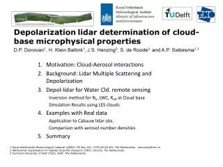
Depolarization lidar for water cloud remote sensing. Background: MS and Depolaization Short overview of the MC model used in this work Depol -lidar for Water Cld remote sensing: Model cases Example with Real data Summary. Lidar Multiple scattering. Lidar FOV cone. 1 st order.

E N D
Depolarization lidar for water cloud remote sensing Background: MS and Depolaization Short overview of the MC model used in this work Depol-lidar for Water Cld remote sensing: Model cases Example with Real data Summary
Lidar Multiple scattering Lidar FOV cone 1st order 4th order total 2nd order 3rd order Photons can scatter Multiple times and remain within lidar Field-Of-View Enhanced return w.r.t single scattering theory Scattering by cloud droplets of At uv-near IR is mainly forward
Multiple Scattering induced depolarization • For a polarization sensitive lidar MS also gives rise to: • A Cross-polarized signal even for spherical targets. • Depends on: • Wavelength • Size Dist.(Reff profile) • Extinction profile • Filed Of View • Distance from Lidar In order to calculate MS enhanced signal and depol accurately Monte-Carlo approaches must be used.
What is a MC simulation ? (simple example with no variance reduction techniques) Launch Photon packet Determine path length until next interaction using PRNG and Beer’s law Determine scattering angle using PRNG and scatterer’s phase function Loop until packet is absorbed, hits receiver or migrates too far from the receiver fov Loop in packet until desired SNR is reached
ECSIM lidar Monte-Carlo model • MC lidar model developed originally for EarthCARE (Earth Clouds and Aerosol Explorer Mission) satellite based simulations. • Uses various “variance reduction” tricks to speed calculations up enormously compared to direct simple MC (but is still computationally expensive). • Capable of simulations at large range of wavelengths and viewing geometries, including ground-basedsimulations.
Validation: Against other MC models and Observations ECSIM vs other MC results Validation (vs other models): Cases presented in Roy and Roy, Appl. Opts. (2km from a C1 cumulus cloud OD=5) Circ lin ECSIM MC results Carswell and Pal 1980: Field Obs. Roy et al. 2008: Lab results
Connection towater cloud remote sensing…. Not too long ago, motivated by the observations of highly depolarizing volcanic ash I was looking for a way to verify the depol. calibration of a lidar system I operate. Motivated by Hu’s results for Calipso, I wondered if Strato-cu could be a good target So I setup a script to run my MC code on several hundred cases using a simple water cloud model (Fixed LWC slope and Constant N) The results were initially disappointing…..the resulting depol and backscatter relationships depended too much on the LWC slope and N ! Hmmm….. maybe I should look at this in some more detail from the other side.
Some Examples: A simple water cloud model is used: Adiabatic Linear LWC profile and constant number density
D_LWC/dz = 0.5 gm-3 D_LWC/dz = 1.0 gm-3 Para Profiles normalize so that the peak is 1.0 Look-up-tables were made for several cloud-bases, different size-dist widths and receiver fovs.
Same extinction profile but different Reff profiles Depol and `Shape’ largely a function of extinction profile but exploitable differences exist, especially at small particle sizes (depends somewhat of fov). However at larger effective radii values then there is no size sensitivity.
Trial using one of the `blind-test’ LES scenes WITH DRIZZLE !
Since effectively only information from the lowest 100 meters of the clouds is used. Departures from “good behavior” particularly near cloud top are problematic.
A case using real data A real case: Cabauw: Leosphere ALS-450 355nm, 2.3 mradfov
Comparison with uwave radiometer observations and sensitivity to size-dist width assumptions , fov and depol calibration uncertainties Ran out of time… ….but preliminary findings are encouraging.
Summary • Lidar Depolarization measurements are an underutilized source of information on water clouds. • Fundamental Idea is not new…Sassen, Carswell, Pal, Bissonette, Roy, etc… have done a lot of work stretching back to the 80’s and likely earlier. • But now with better Rad-transfer codes and much faster computers a re-visit is in order.
The general problem (i.e. the inversion of backscatter+depol measurements to get lwc profile and Reff under general circumstances ) is complex and likely requires multiple fov measurements. However… • Constraining the problem to adiabatic(-like) clouds simplifies things and enables one to construct a simple and fast inversion procedure. Still early days but the idea looks worth pursuing. There is A LOT of existing lidar observations it could be applied to. • Results are insensitive to presence of drizzle drops ! • Lots of opportunities for synergy with radars, uwave radiometers and other instruments. • Will require some thinking on how to integrate within an Ipt-like scheme.